Gaussian Processes

for the General Practitioner

Benjamin Pope

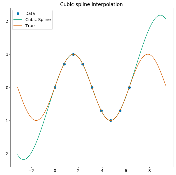
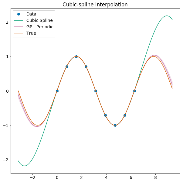
Interpolation

We often want to model a function - say, an image, or a time series - where we might not be able to specify some functional form in advance, but rather only very general properties, such a a rough amplitude and length scale.

When we interpolate, we are performing a regression analysis, trying to fit a function to data. This is the same problem as extrapolation, where we are predicting the value of this function a long way from the samples on which it is conditioned.

Interpolating with splines

Splines are a common piece-wise polynomial model, anchored at a finite set of points, used for interpolation.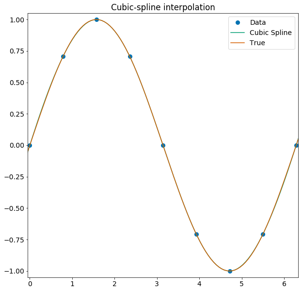

These are no good for extrapolation. We need something that won't blow up away from the data!

Gaussian Processes

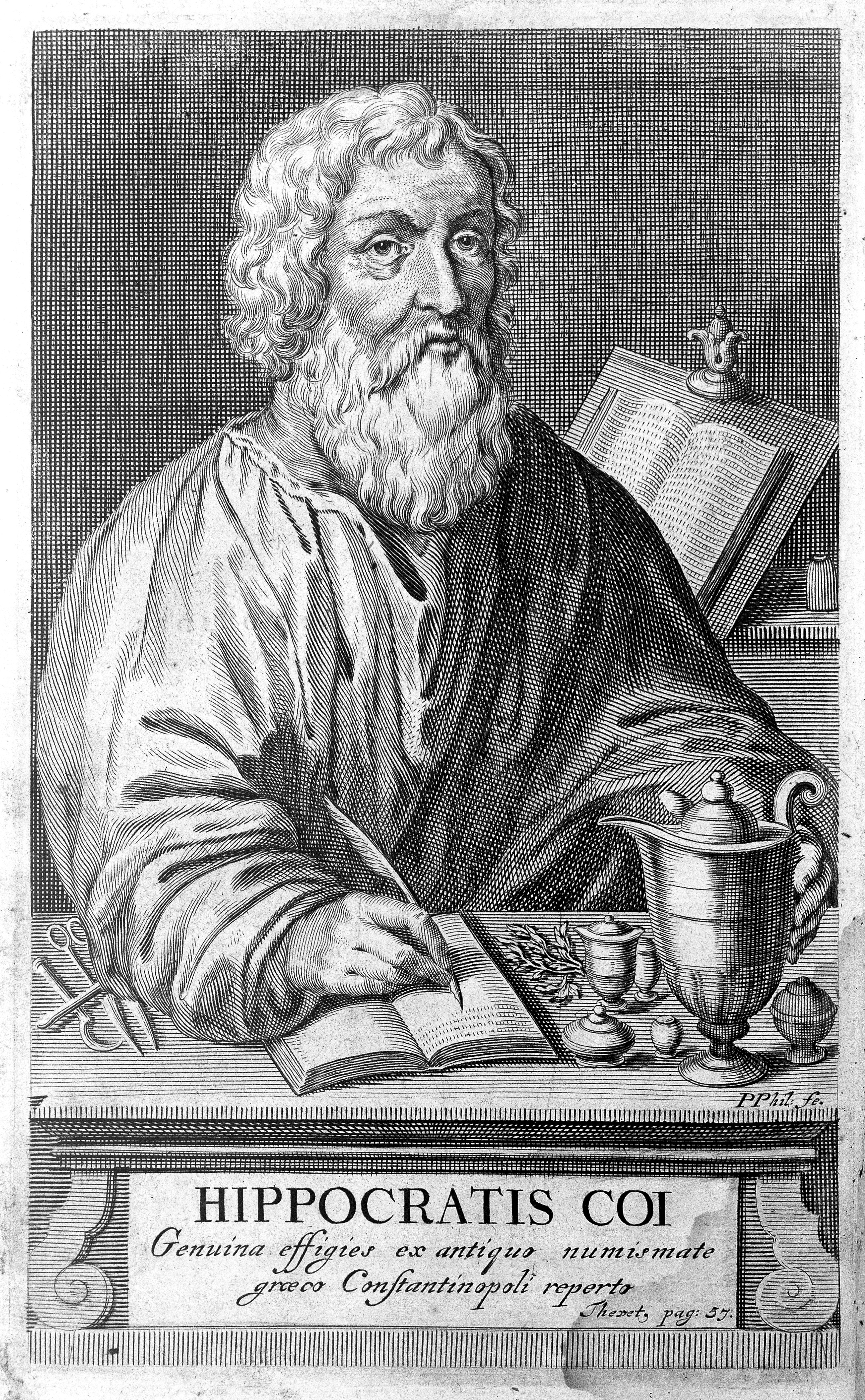
Hippocrates: 'First, do no harm'.

Go to a GP - a Gaussian Process!

A Gaussian Process is a distribution over functions such that any finite set of samples are jointly Gaussian-distributed.

These are sometimes also referred to as Gaussian random fields.

\[ \underbrace{\mathbf{y}}_{\text{data}} \sim \mathscr{N}(\overbrace{\mu}^{\text{mean}},\underbrace{\mathbf{K}}_{\text{covariance}}) \]

These are good for regression where you have some idea of the shape of a function, and crucially, give you estimates of the uncertainty in your predictions as well.

You specify a mean function \[\mu(\mathbf{x},\mathbf{\theta}_\mu) \] which defines a deterministic, parametric model (e.g. the orbit of a planet)...

and a covariance function \[\mathbf{K}(\mathbf{x}_1, \mathbf{x_2}, \mathbf{\theta}_K) \] which generates random variations, such as stellar activity.

In general you will want your covariance function to simply be a 'kernel' \[\mathbf{K}(x_1,x_2) = k(|\mathbf{x}_1 - \mathbf{x}_2|, \mathbf{\theta}_K) \]

which we see depends only on the distance between your input data.

Any zero-mean GP/Gaussian Random Field is fully characterized by its power spectral density (PSD), or equivalently, its covariance function.

These are interchangeable because of the Wiener-Khinchine theorem, which states that these are related by a Fourier transform.

\[ \underbrace{f\star f}_{\text{autocorrelation}} = FT(|f|^2) \]

These can be simple 1D functions, like here where \(k(\Delta t) = \exp(-{\Delta t}/\tau)^2 \)

... or these can have higher dimensions. For example, the Kolmogorov theory of turbulence has a self-similar, power-law power spectral density in wavenumber \(k\)

\[ E(k) \propto k^{-5/3} \]

which generates the Gaussian Random Field below. Kolmogorov Turbulence

You can use GPs to interpolate conservatively!

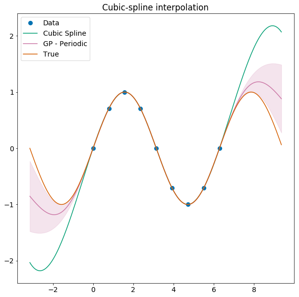
... and work better if you optimize the kernel.

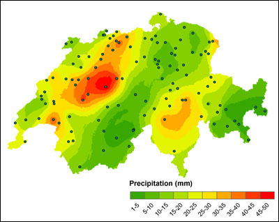
History

Danish astronomer Thorvald Thiele was the first to my knowledge to use something like a GP, discovering what was later called the Kalman Filter, a special case of the GP.

GP filtering was rediscovered in similar but different forms by American Norbert Wiener in the context of controlling anti-aircraft guns in World War II, and contemporaneously by Andrey Kolmogorov in the Soviet Union. This inspired Rudolf E. Kálmán to develop the Kalman filter for missile guidance in the Cold War.

Matheron defined 'kriging' (after pioneering miner Danie Krige) as a technique in geospatial statistics 'computing the weighted average of available samples... The suitable weights \(a_i\) are determined by \(\sum_i a_i = 1 \)... [and the prediction] variance... should take the smallest possible value'.

The idea was that if it is expensive to take exploratory samples, you should have some optimal interpolating method that knows about the spatial structure of an ore body to help you make the best inference about where to mine.

This has also been used in meteorology, to interpolate between a few weather stations across a wide region (eg Switzerland below)

http://www.gitta.info/ContiSpatVar/en/html/Interpolatio_learningObject3.xhtml

GPs are now ubiquitously used in machine learning: 'Bayesian neural networks with infinitely many hidden units converge to Gaussian processes with a particular kernel (covariance) function' (from here and here). Serious machine learning people are trying to combine the smoothness and power of GPs with the flexibility of neural networks - this is a hot topic!

So how does it work?

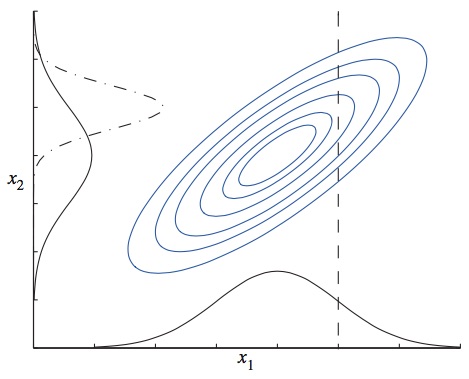
Information about \(x_1\) tells you more about \(x_2\) than just the marginal distribution - because they are correlated, learning \(x_1\) allows you to predict \(x_2\) more accurately.

In using a GP we exploit this by knowing the correlations across, say, a whole time series or spatial map.

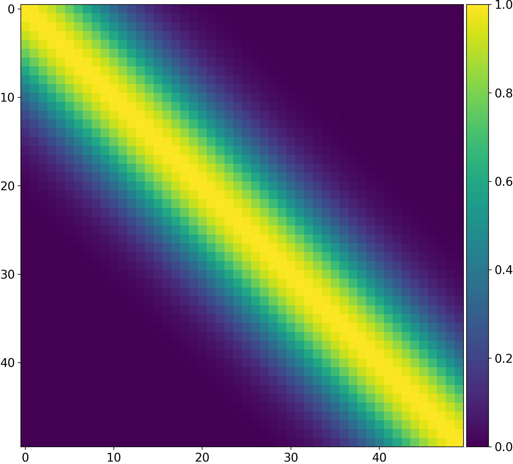
This is characterized by a covariance matrix like this, for squared exponential correlation with \(\lambda = 100\).

Remarkably, the posterior for a GP conditioned upon data \(\mathbf{x}_* \) is also a GP, and has an analytic distribution

\[ p(\mathbf{y}*) = \mathscr{N}(\mathbf{m}_*, \mathbf{C}_*),\]

where \[ \mathbf{m}_* = \mathbf{\mu}(\mathbf{x}_*) + \mathbf{K}(\mathbf{x}_*, \mathbf{x})\mathbf{K}(\mathbf{x}, \mathbf{x})^{-1} (\mathbf{y}(\mathbf{x}) - \mathbf{\mu}(\mathbf{x})) \]

and
\[ \mathbf{C}_* = \mathbf{K}(\mathbf{x}_*,\mathbf{x}_*) -\mathbf{K}(\mathbf{x}_*,\mathbf{x})\mathbf{K}(\mathbf{x},\mathbf{x})^{-1}\mathbf{K}(\mathbf{x}_*,\mathbf{x})^T. \]

Implementing a GP

1. Choose your mean function \(\mu(\mathbf{x},\mathbf{\theta}_\mu)\) and kernel \(k(\mathbf{x},\mathbf{\theta}_k)\) appropriate to the problem.

2. Fit your kernel hyperparameters \(\mathbf{\theta}_k\). This is usually too expensive to jointly fit with your deterministic model.

3. Compute your GP covariance matrix. This is now just a familiar \(\chi^2\) problem.

4. MCMC to get posteriors for the parameters \(\mathbf{\theta}_\mu\).

Choosing your kernel

Your kernel can be thought of as matching the impulse response function of a linear system. So for a driven, damped harmonic oscillator, the kernel is

\[ k(\Delta t) = A_0 \cdot \exp{(-\dfrac{\Delta t}{\tau})} \cos(\omega \Delta t) \]

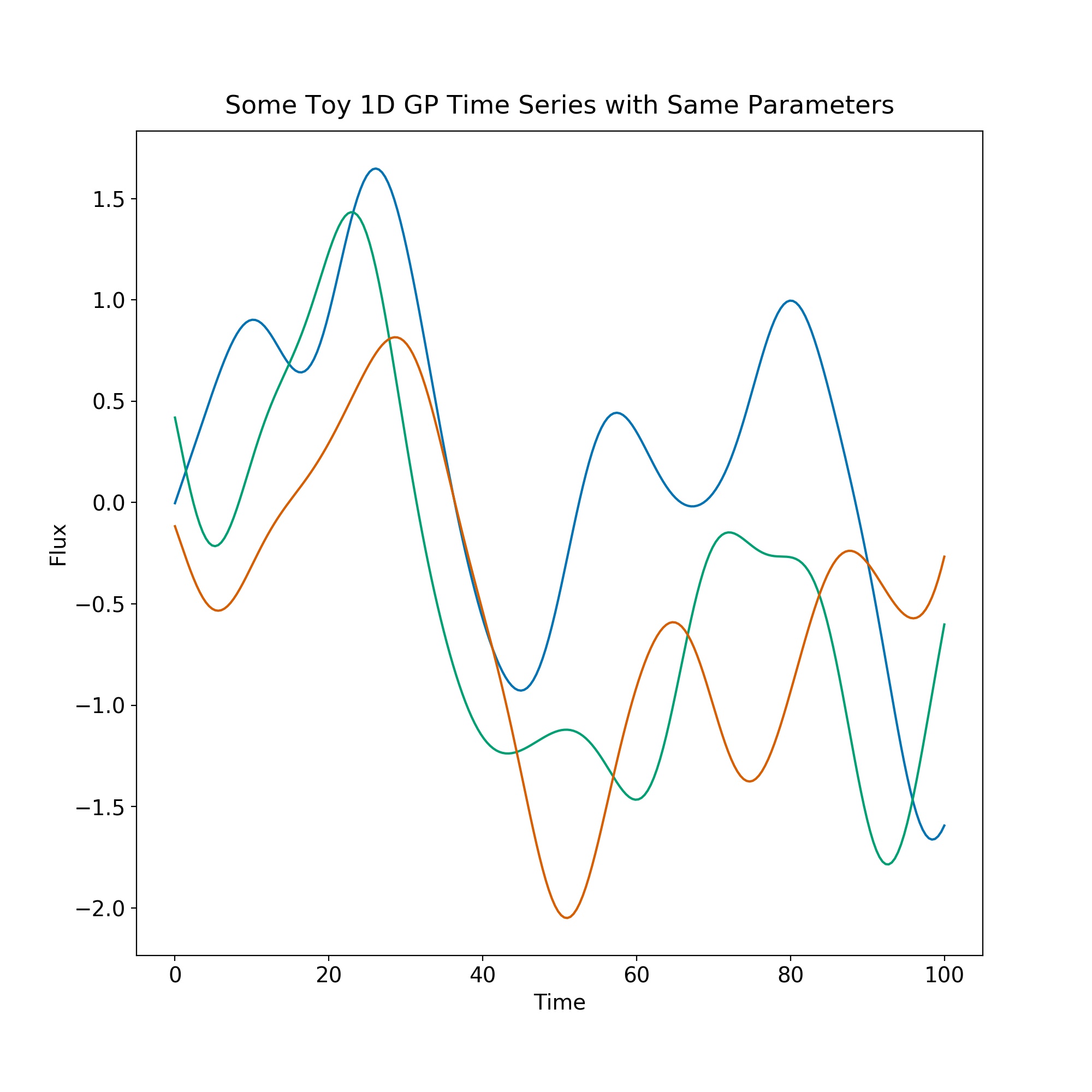
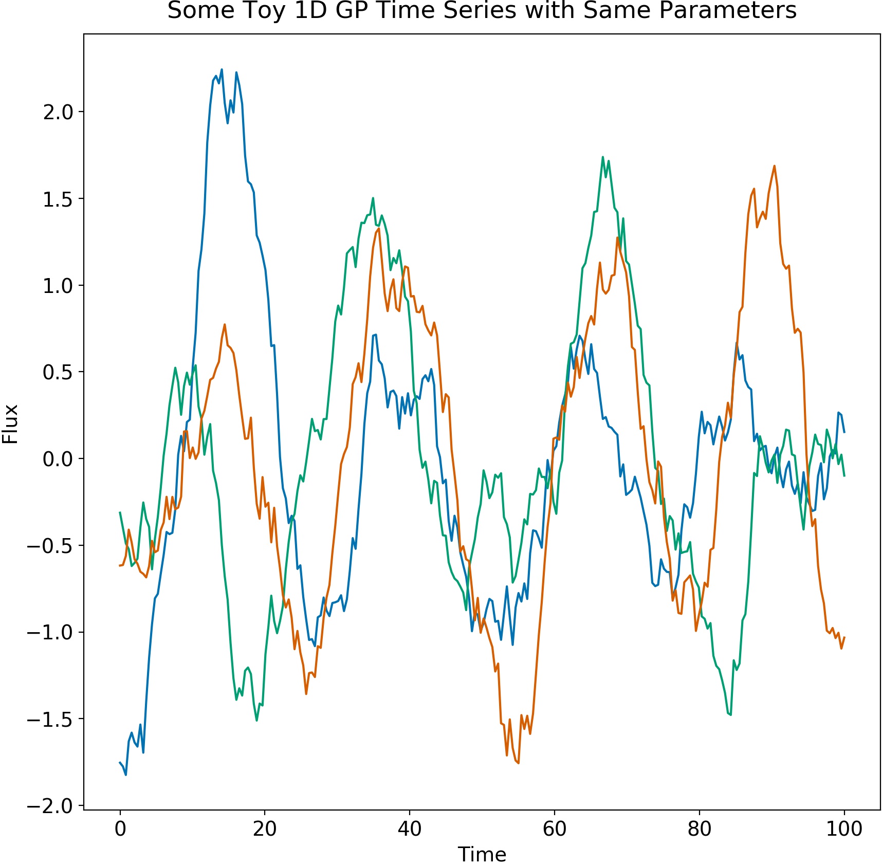
Let's look at some draws from this distribution.

There are many kernels for different tasks, and I will not cover them all here. For example, there is the Matern-3/2 kernel

\[k(r^2) = (1+\sqrt{3r^2}) \exp(-\sqrt{3} r^2) \]

which is good for rough or jagged processes.

Or there is the Exponential Sine Squared kernel

\[k(x_i,x_j) = \exp(-\Gamma \sin^2{(\dfrac{\pi}{P} |x_j - x_i|)})\]

which is good for periodic processes which 'lose memory' at a rate determined by \(\Gamma\).

Choosing the kernel is often as much an art as a science - while it should ideally match the dynamics of the system, in practice these are often not well known, and a combination of experimentation and intuition is required.

Often you will want to represent white noise as a diagonal term in your covariance matrix, so that

\[\mathbf{K} = \mathbf{K}_0 + \sigma^2 \mathbf{I}. \]

This white noise parameter \(\sigma\) allows you to account for uncorrelated errors safely.

Hyperparameters

The parameters \( \tau, P, \Gamma, \nu\) et cetera above are called hyperparameters.

While GPs are non-parametric models, the general information such as length scale, period, amplitude and so forth that controls a GP is determined by these hyperparameters. In general, you will want to optimize these to get the best possible fit to your data.

Conveniently, the GP has an analytic marginal likelihood!

\[ \log p(\mathbf{y}|\mathbf{x},\mathbf{\theta},I) = -\underbrace{\dfrac{1}{2} \mathbf{y}^T (\mathbf{K}+\sigma^2 \mathbf{I})^{-1} \mathbf{y}}_{\text{data fit}}\]

\[-\underbrace{\dfrac{1}{2} \log(\det(\mathbf{K}+\sigma^2 \mathbf{I}))}_{\text{complexity penalty}} - \underbrace{\dfrac{n}{2}\log(2\pi)}_{\text{constant}]\]

You will usually use an optimizing library such as scipy to maximize the likelihood of this GP fit and therefore optimize the hyperparameters - you uually don't care as much about their detailed distribution.

In practice the determinant and matrix inversion are what kills you, as these scale as \( \mathscr{O}(3)\) with the number of data points \( n\) - brutal!

It is very often the case that most of the ingenuity in a GP software package is in implementing a clever matrix decomposition such as the HODLR or Cholesky decompositions, which are beyond my mortal ken.

There are excellent GP packages available to do this, such as george, celerite, scikit-learn, and pyGPs, which are all fast and stable.

Examples

Spectral Line

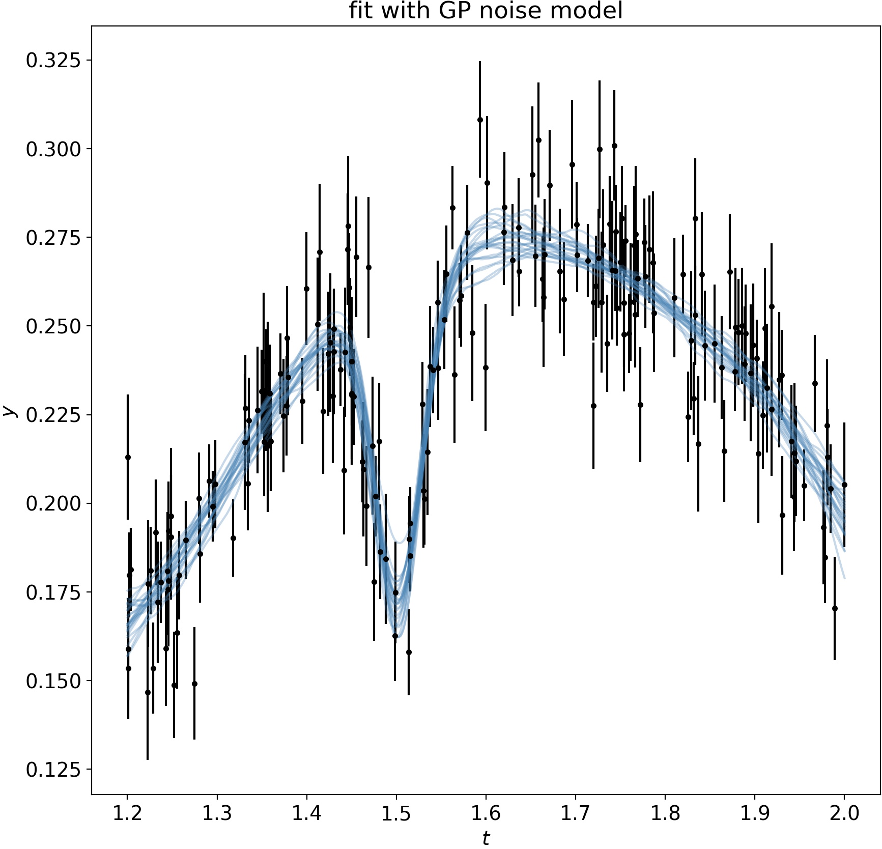
A Test Case

Very often the gain on a radio telescope can vary considerably across a spectral bandpass, due to interference or imperfections in the electronics. We are going to look for a Gaussian spectral line amid correlated noise across the spectral band.

Remember the mean function? We can use a GP to account for correlated noise.

You jointly fit the mean parameters \(\mathbf{\theta}_\mu\) and the stochastic parameters \(\mathbf{\theta}_K\) with, say, MCMC or nested sampling.

We have generated data with a real spectral line at 1.5 GHz, with depth 0.1, and \(\log(\sigma^2) =0.0005 \), buried in correlated noise from a GP with a squared-exponential kernel, \(\lambda=0.5\), amplitude 0.1.

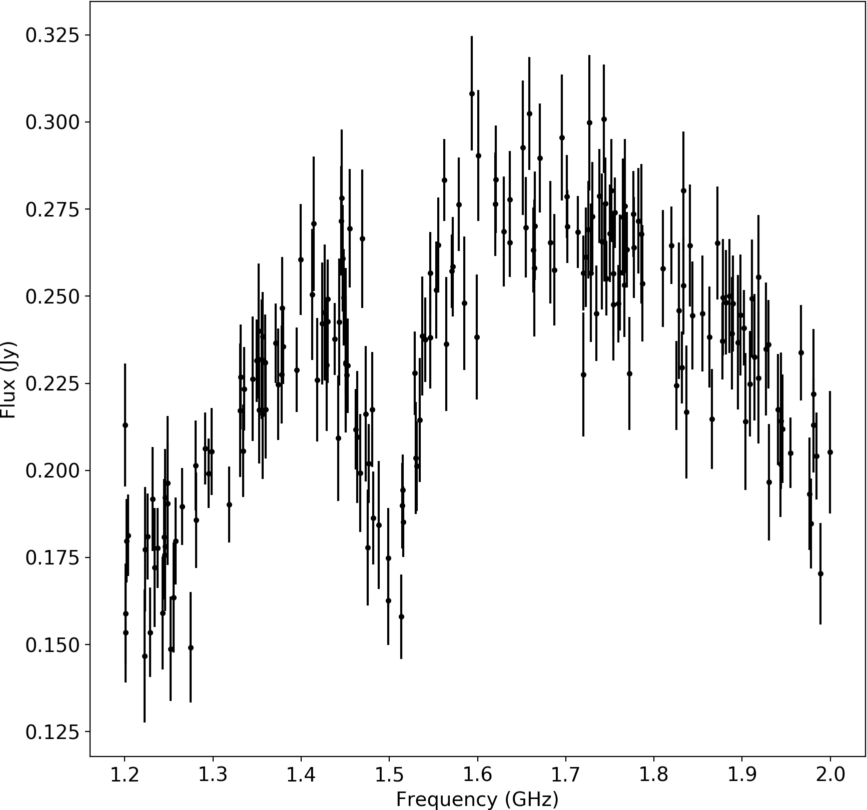
Not knowing the true kernel, we want to infer the parameters of the line buried in this correlated noise. Using george to model our GP, we choose a Matern-3/2 kernel - we shall see that the mismatch in kernel isn't too bad.

Using emcee, an affine-invariant MCMC sampler, we fit the GP hyperparameters jointly with our Gaussian line model.

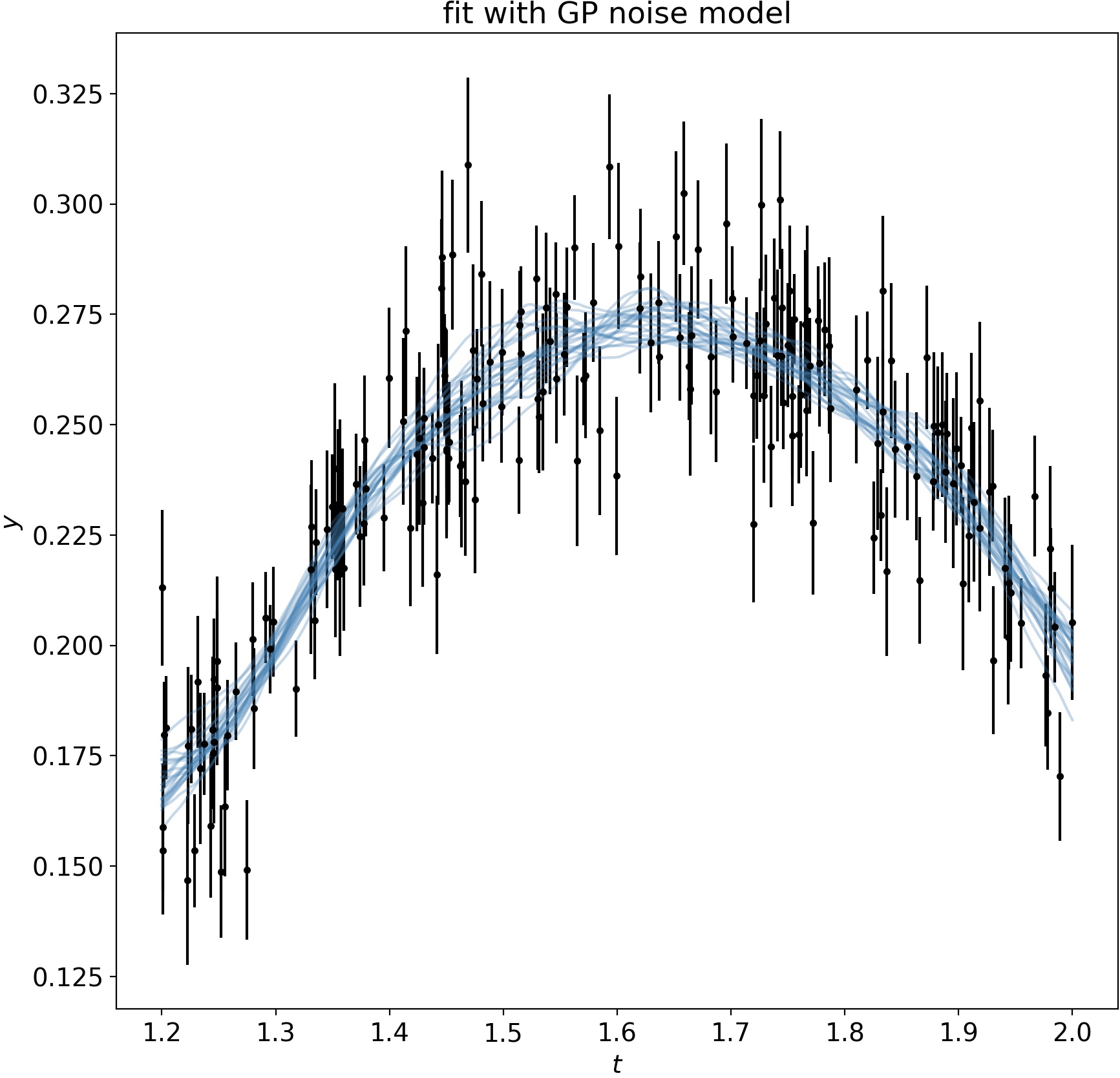
We can subtract the best model fit out to see how well the GP models the noise:

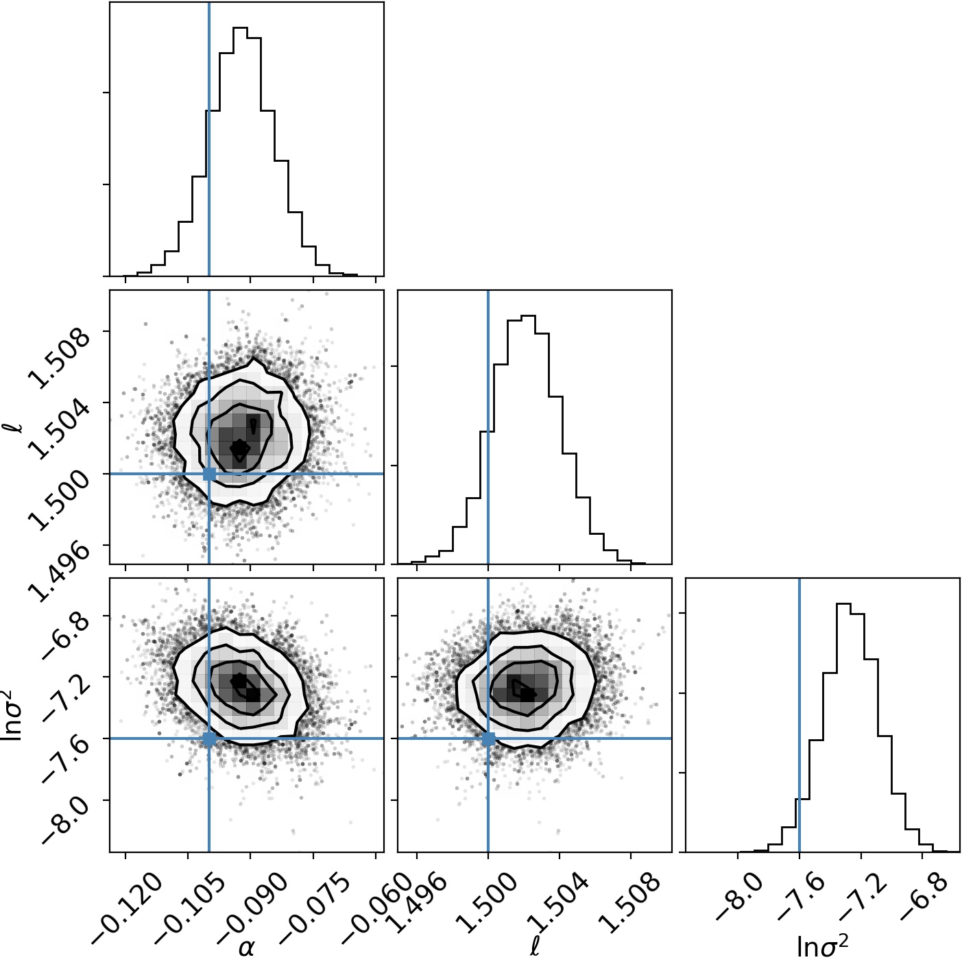
And we can make a corner plot to show the marginal distribution we get for the model parameters. We nail it pretty well in some tough noise!

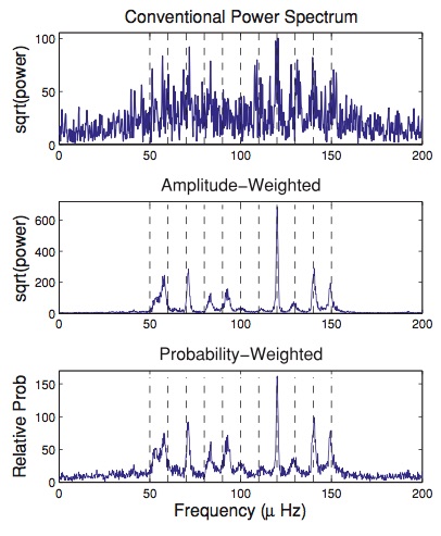
Asteroseismology

In asteroseismology, a star rings like a bell and its frequencies tell us important information about the stellar interior.

For solar-like stars driven by convective noise, the signal should reduce to a sum of simple harmonic oscillator Gaussian Processes. \[ k(\Delta t) = A_0 \cdot \exp{(-\dfrac{\Delta t}{\tau})} \cos(\omega \Delta t) \]

Brewer & Stello, 2009.

Multiple Inputs and Outputs

A GP kernel can depend on several different inputs (eg position and time), and a GP can output a vector-valued function.

Searching for Exoplanets

Exoplanets are detectable by the dip they cause in brightness as they pass in front of a star...

... but the instrument is not perfect, and stars can vary for other reasons!

Exoplanet-style transit light curve of Venus from James Gilbert on Vimeo.

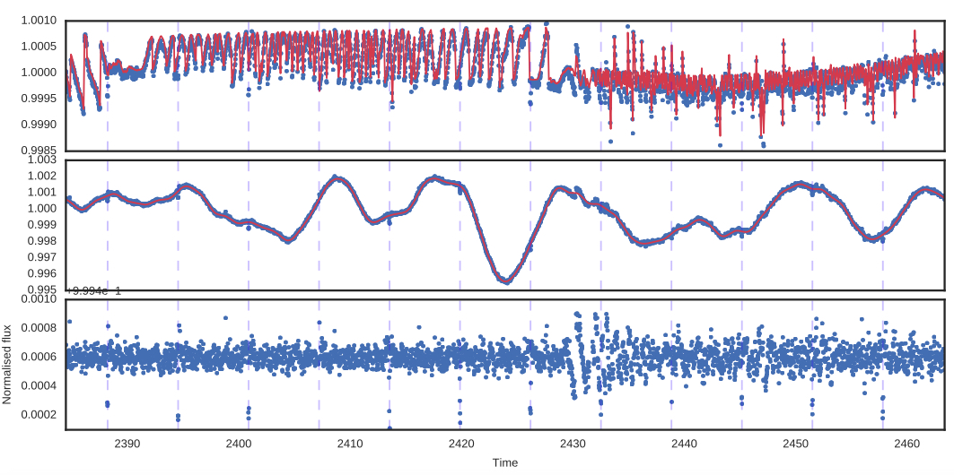
Raw K2 Data

So we model this as a 2D GP: with a squared exponential kernel in both time and in the spacecraft roll angle.

We calibrate out the error introduced by roll by then predicting the GP at each roll angle, with time set to zero - and subtract this purely-roll systematic from the real data.

Aigrain et al., 2015.

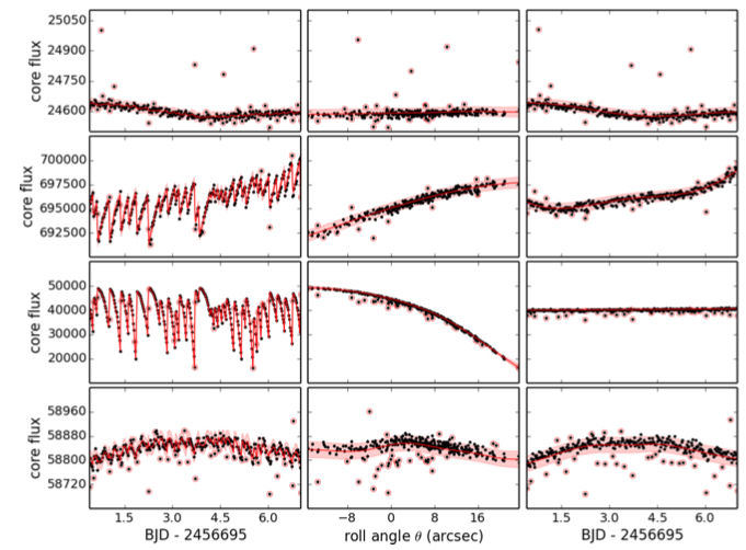
A planet - EPIC 212357477 b

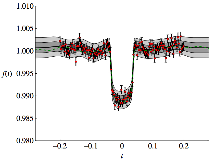
http://www.robots.ox.ac.uk/~sjrob/Pubs/philTransA_2012.pdf

Roberts et al., 2012 want to infer \(\mathbf{\theta}_\mu\) (orbital parameters, planet radius, etc) and marginalize over instrumental systematics as nuisance parameters.

Traps

Cowtan & Way (2013) realised that there was very poor coverage of temperature maps near the poles – only 84% global coverage.

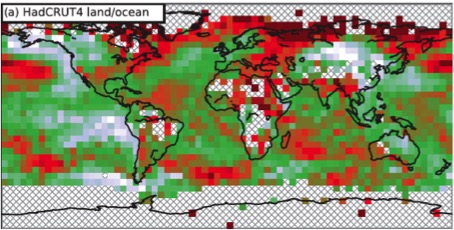
If you use a GP to try and fill in the gaps, you find there has been a bias to estimating lower global warming than previously thought.

The issue is that the poles have very different physics to the equator and you can't interpolate one over the other - GPs model stationary processes!

Conclusions