STScI Colloquium: Benjamin Pope

The Brightest Stars

and their Planets

Benjamin Pope, NYU

Slides available at
benjaminpope.github.io/talks/stsci/stsci.html

Transiting Planets

Large searches for exoplanets like the Kepler mission have shown planets to be common in our Galaxy - now we want to learn about their atmospheres and compositions.

Atmospheric spectra can come from transmission spectroscopy during a transit, or direct imaging at high contrast and angular resolution.

For transmission spec, the best options are those around bright stars, like 55 Cancri e - subject of 367 papers in the last decade!

My Sagan Fellowship project is to search for planets transiting naked-eye stars (V mag < 6.5) in order to find ideal targets for characterization with the upcoming James Webb Space Telescope.

For direct imaging I have helped develop and apply the kernel phase method to HST and JWST data, to improve contrast achievable at angular resolutions of \(0.5 \lambda/D\)

I am both a data scientist and an optical physicist - combining optical theory and statistics lets us get the most out of each instrument

Kepler Photometry

After the failure of a reaction wheel in 2012, Kepler was rebooted as the 'K2 Mission', with very unstable pointing (hence the shaking in the videos you'll see).

To get the photometry, you can just sum the pixel values in a window containing the whole PSF...

but the pixels have different gains ("inter- and intra-pixel sensitivity variation")...

and the pixel window doesn't necessarily track the whole PSF perfectly ("aperture losses").

For sufficiently bright stars light fills the CCD wells with electrons that spill up and down the column and even leaving the chip.

Kepler saturates on stars brighter than ~ 11th mag - but we want to look at 1st mag stars: 10k times brighter!

Halo Photometry

What if we just look at unsaturated pixels?

Flux \(f_i \) at cadence i is a sum over j pixels \(p_{ij}\) with weights \(w_j\):

\[ f_i \equiv \sum\limits_j w_j p_{ij} \]

To find the appropriate weights, minimize the Total Variation

\[\begin{align} TV \equiv \sum_i |f_i - f_{i-1}| \end{align} \] subject to constraints \[\begin{align}\forall_j w_j &> 0\\ \sum_{i=1}^{N} f_i &= N.\end{align} \]

This is the \(L_1\) norm or 'taxicab metric' on the derivative of the time series.

This has analytic derivatives you can compute with automatic differentiation - easy to optimize.

I led the K2 Bright Star Survey: asteroseismology and variability classifications for all 161 stars - a unique legacy sample.

K2 Halo data of the 161 naked-eye stars are available as High Level Science Products on MAST archive.stsci.edu/hlsp/halo

Released pipeline as open source: github.com/benjaminpope/k2halo

Pleiades

Πλειάδες, the Seven Sisters

Alcyone, Atlas (dad), Electra, Maia, Merope, Taygeta, Pleione (mum)

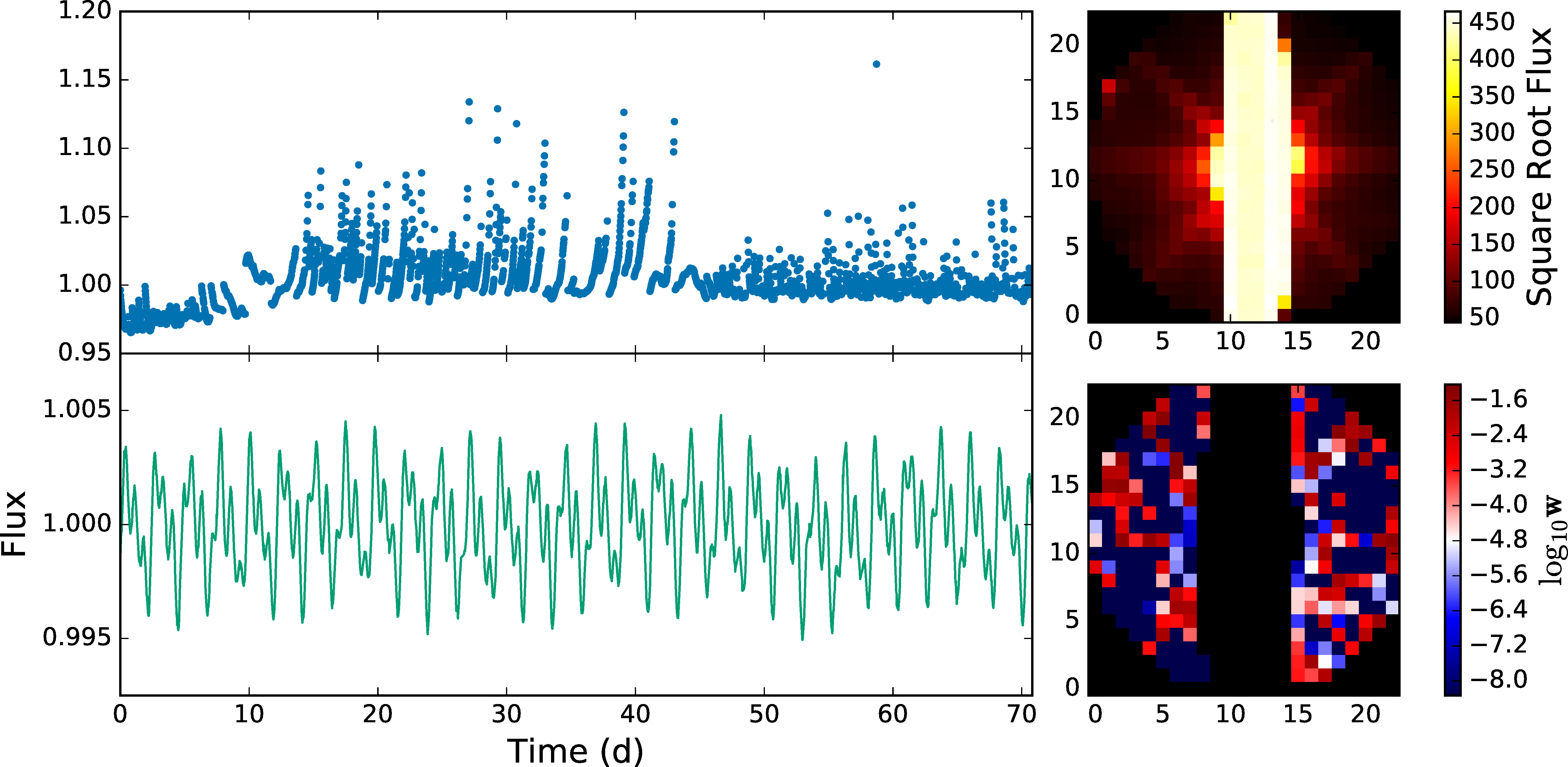
Atlas lightcurve: raw (top) and halo (bottom)

White, Pope et al., 2017

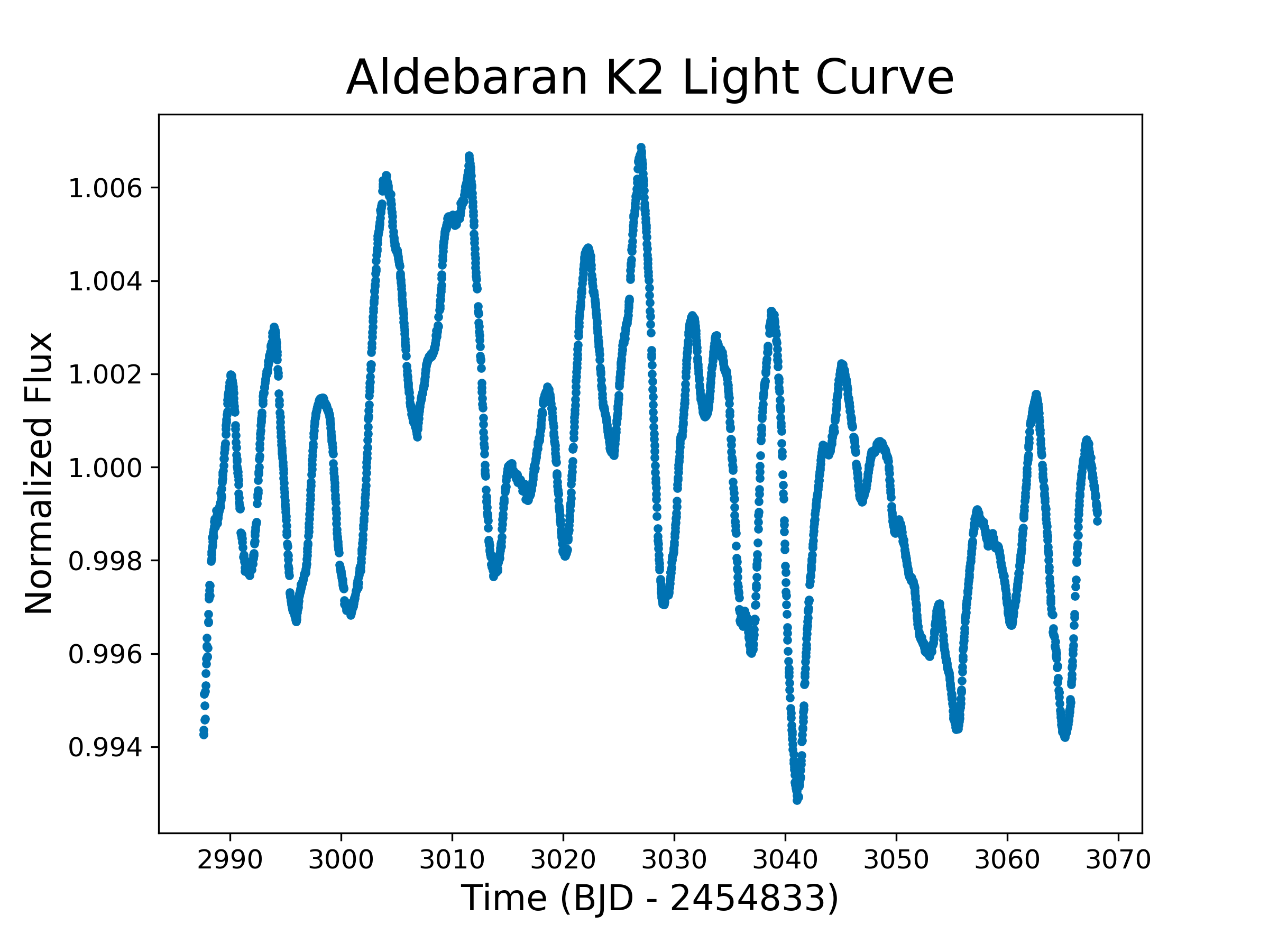
Aldebaran

α Tauri

الدبران ,the follower

... follows the Pleiades!

Hatzes & Cochran, 1993 claimed an early detection of a \(628.96 \pm 0.90\) d RV planet around Aldebaran - finally confirmed in Hatzes et al., 2015!

Detection of p-mode oscillations at 2.2 μHz

Without this asteroseismology, we have

\[M = 1.27^{+0.24}_{-0.20} \, \mathrm{M_{\odot}}\] and age \(4.9^{+3.6}_{-2.0} \, \rm Gyr \)

With this new constraint, I calculated

\[M = 1.16^{+0.07}_{-0.07} \, \mathrm{M_{\odot}}\] and age \(6.4^{+1.4}_{-1.1} \, \rm Gyr \)

Using MESA models, I found that on the main sequence Aldebaran b had a semi-major axis of \(1.50 \pm 0.03 \) AU and Aldebaran had a luminosity \(2.0 \pm 0.7 \, L_\odot \)...

so Aldebaran b had an insolation comparable to Earth when its star was on the main sequence. First dead planet!

This halo method is now successfully being applied to TESS - debunking a spurious transit candidate around τ Ceti (Eisner, Pope et al 2019) and for asteroseismology of many bright stars such as α Cen AB and β Hyi (in prep!)

Direct Imaging

We are starting to detect planets at the epoch of formation - eg the accreting protoplanets PDS 70 bc.

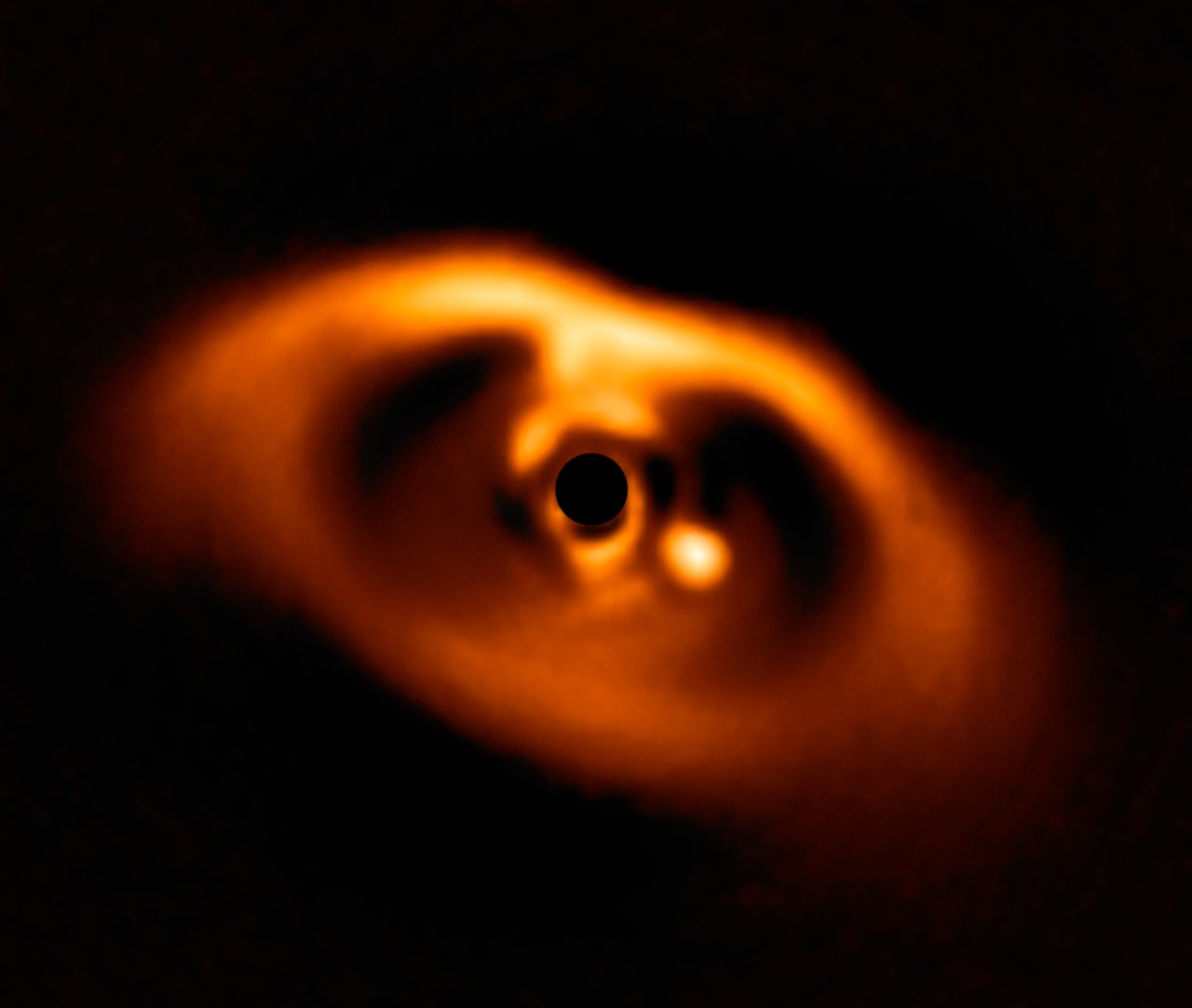
(ESO/A. Müller et al.)

The main limitation on direct imaging is from wavefront aberrations which corrupt phase information.

In radio astronomy the idea of 'closure phase' was developed to be immune to phase noise:

Correlate baselines around a triangle of receivers

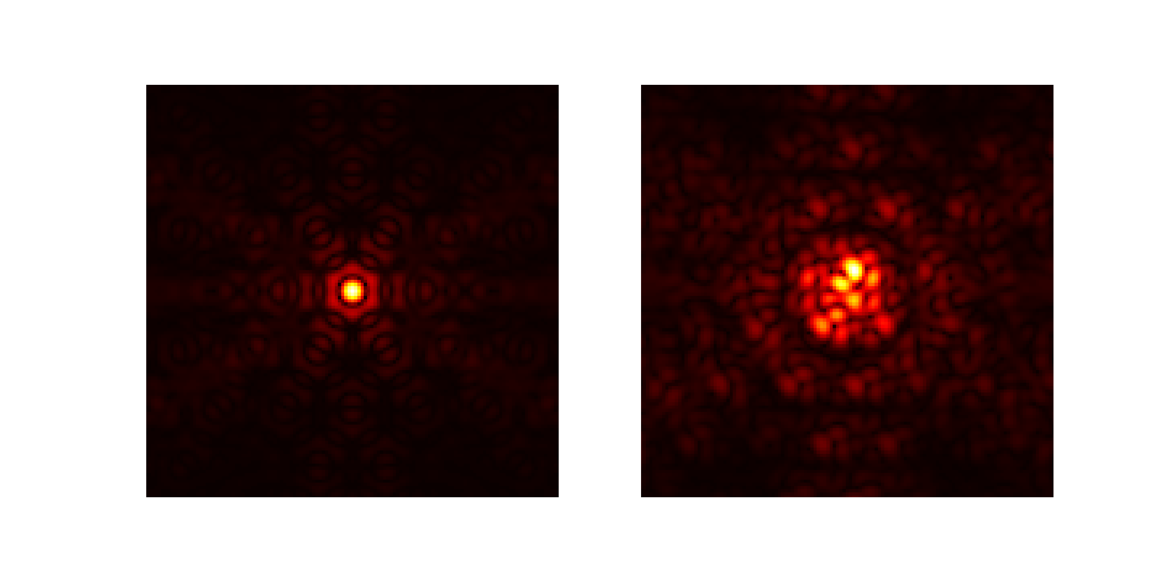
JWST has an aperture masking instrument on NIRISS to obtain closure phases

Kernel phase is a generalization of closure phase to arbitrary pupils.

Linearize response to phase noise: suitable for stable high Strehl images, with point-source calibrators

Separate out linear subspaces of Fourier components that are immune to phase noise vs susceptible

Used this in Pope et al, 2013 to revisit the Reid et al 2006, 2008 HST NICMOS volume-limited brown dwarf surveys and discover 5 additional tight binaries.

The other subspace can be used for wavefront sensing

Every point source image gives you a free wavefront measurement in the instrument pupil!

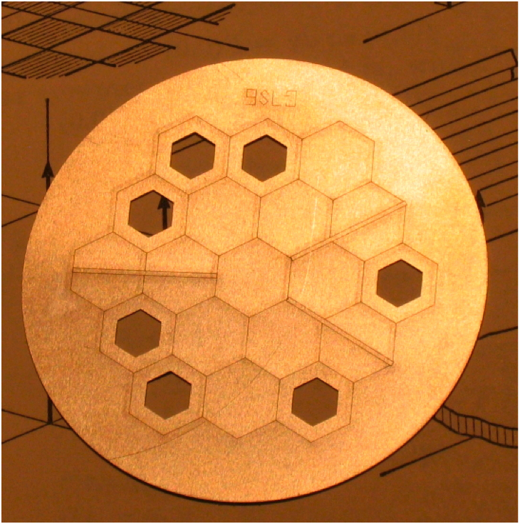
Cophasing segmented mirror in the lab (Pope+2014)

This linearization can be applied to arbitrary optical systems - eg coronagraphs such as JWST-NIRCAM/MIRI and WFIRST.

Optics is mathematically like machine learning: matrix multiplications and simple nonlinear functions

Can use automatic differentiation!

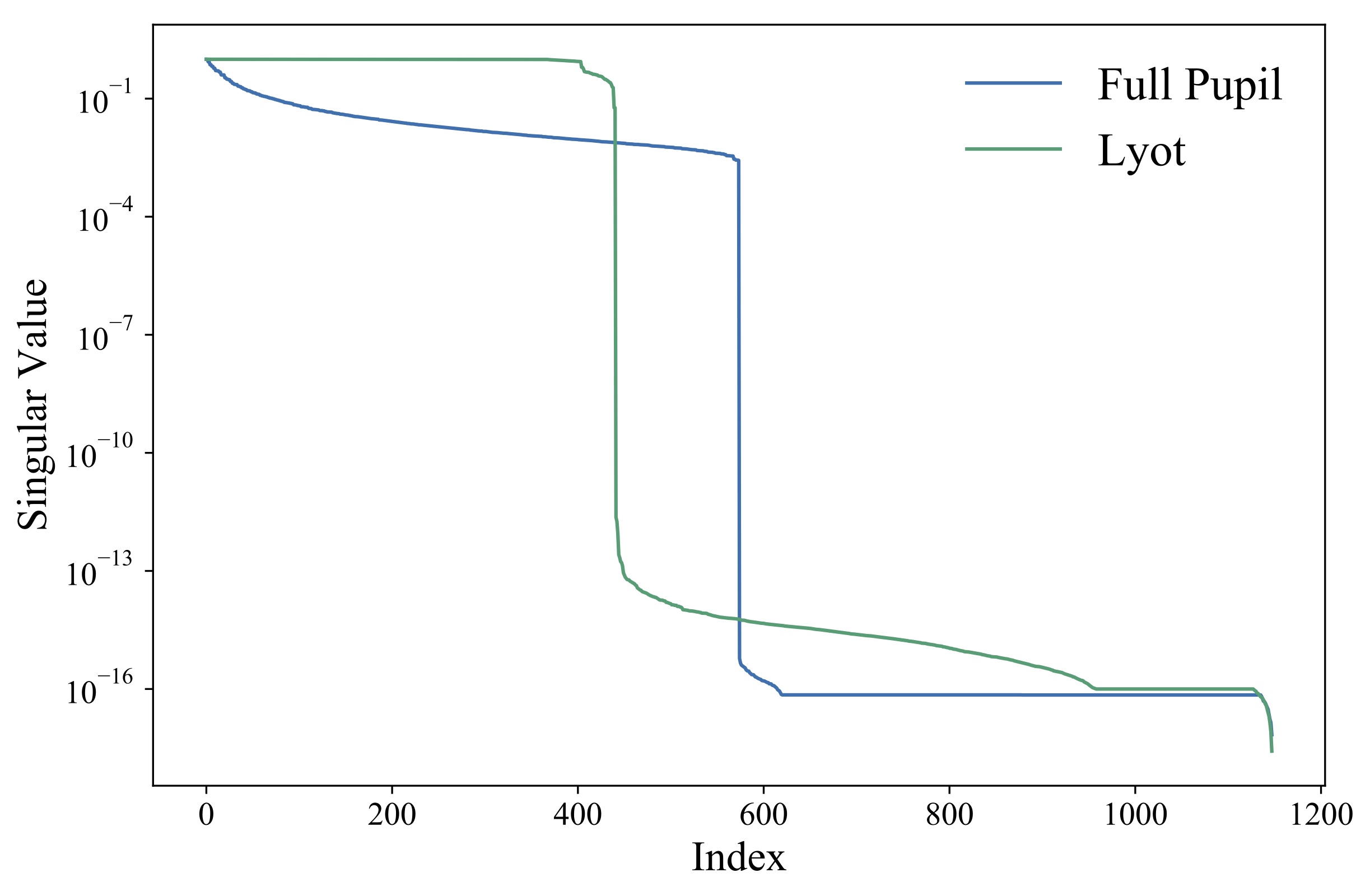
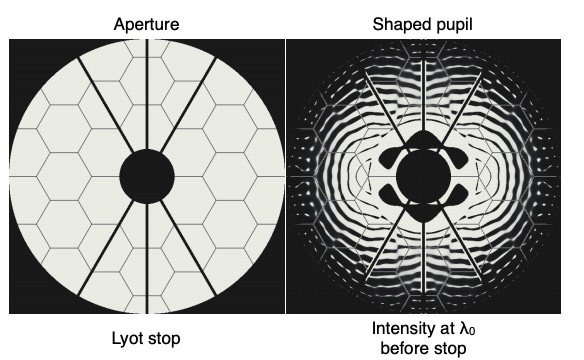
Extending kernel phase to coronagraphy has the same feature of a noise-corrupted space and a kernel space Singular values

Differentiable optics also allows fast gradient descent for optical design - eg coronagraph pupils

N'Diaye et al 2018

The Future

We have looked at all the bright stars in Kepler and K2 - but the TESS mission will deliver hundreds more. Can we find our nearest neighbours?

Automate a kernel phase reanalysis of HST NICMOS archive - and extend to all JWST point sources

What can we do with open data and open software more broadly in astronomy?