Imaging, part 6: sparse images and CLEAN
The regularisers of parts 2 and 3 prefer smooth images. Some scenes are not smooth: a companion or two and a few compact knots next to a bright star. CLEAN (Högbom 1974), the oldest image reconstruction algorithm in radio astronomy, builds an image for such scenes from point sources, one at a time.
Högbom's CLEAN works on the dirty image: it finds the brightest point in the residual dirty image, adds a small fraction (the loop gain) of a point source there to the model, subtracts its dirty beam from the residuals, and repeats. That needs data that are linear in the image, such as calibrated complex visibilities. Closure phases, kernel phases, DISCOs and squared visibilities are not linear, so classic CLEAN cannot use them directly.
virgil's clean uses the same idea in a form that works for any data. For linear data, the residual dirty image is, up to a constant, minus the gradient of χ² with respect to the flux of a point source at each pixel. JAX computes that gradient for any likelihood. So each iteration of clean:
1. computes the gradient of χ² with respect to the flux at every pixel;
2. picks the pixel where a step would lower χ² the most;
3. adds the loop gain times that (Gauss–Newton) step there;
4. stops when χ² per data point reaches one, the discrepancy principle of part 2.
For linear data this is exactly Högbom's CLEAN. Mathematically it is matching pursuit. Step 2 normalises the gradient by how strongly each pixel affects the data. Without that, CLEAN would pile flux into pixels right next to the star, whose light is nearly indistinguishable from the star's own.
This part reconstructs a companion and a knot from AMI DISCOs, refines the result, looks at the loop gain, and then uses closure phases and V² from a long-baseline interferometer.
import sys
from pathlib import Path

import jax
import jax.numpy as jnp
import matplotlib.pyplot as plt
import numpyro.distributions as dist

repo_root = Path.cwd()
if not (repo_root / "src").exists():
    repo_root = repo_root.parent
if str(repo_root / "src") not in sys.path:
    sys.path.insert(0, str(repo_root / "src"))

from virgil.coverage import ami_grid_record, vlti_oidata
from virgil.fitting import fit
from virgil.imaging import (
    beam,
    clean,
    convolve_beam,
    dirty_image,
    field_of_view,
    image_priors,
)
from virgil.likelihood import whitened_residuals
from virgil.models import Image, PointSource, System, circular_support
from virgil.oidata import OIData
from virgil.plotting import (
    plot_data_model_correlation,
    plot_model,
    plot_residual_map,
)
from virgil.scenes import gaussian_blob

# A star with a 2% companion and a 1% knot, both on pixel centres.
template = OIData(ami_grid_record(wavelength_m=4.8e-6, rotation_deg=-6.9))
npix, scale = 40, 20.0
fov = npix * scale
truth = System(
    star=PointSource(),
    companion=PointSource(dra=-90.0, ddec=70.0, flux=0.02),
    knot=PointSource(dra=130.0, ddec=-110.0, flux=0.01),
)
data = template.with_model(truth, key=jax.random.PRNGKey(4))
resolution = beam(data)
print(
    f"{data.n_independent} DISCO coefficients; beam {resolution.major_mas:.0f} × "
    f"{resolution.minor_mas:.0f} mas; {npix}² pixels of {scale:.0f} mas; "
    f"the truth has χ²/N = {jnp.mean(whitened_residuals(truth, data) ** 2):.3f}"
)
588 DISCO coefficients; beam 154 × 131 mas; 40² pixels of 20 mas; the truth has χ²/N = 0.989
The dirty image
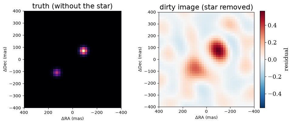
The truth is shown without the star, which would swamp it. The dirty image (part 2), with the star removed, shows the two sources as blurred peaks surrounded by the sidelobes of the dirty beam. CLEAN's job is to replace those patterns with the point sources that made them.
dirty = dirty_image(data, npix, scale, flux_ratio=0.03)
fig, axes = plt.subplots(1, 2, figsize=(10, 4.2))
faint = System(companion=truth.companion, knot=truth.knot)
plot_model(faint, fov_mas=fov, npix=npix, ax=axes[0], title="truth (without the star)")
plot_residual_map(dirty, fov, ax=axes[1], title="dirty image (star removed)")
plt.tight_layout()
plt.show()
Running CLEAN
clean(data, npix, pixel_scale_mas, base=...) adds components to a fixed base scene, here the star, with flux 1. Fit the base's parameters first if it has any. The component fluxes are relative to the base, like a companion's flux in a System.
The support says where components may go. A hole of half a beam under the star stops CLEAN trading the star's flux against the pixels around it, as starting_image does in part 2. The loop gain is 0.1 by default.
Each iteration only adds flux. Every refit_every iterations (50 by default) a major cycle, as in the Clark and Cotton–Schwab variants of CLEAN, refits the fluxes of all the components at once, keeping them non-negative. Flux can then move off an early mistake, and a component whose flux falls to zero is removed.
CLEAN stops when χ² per data point reaches target_chi2_red, 1 by default. That target assumes the error bars are right. Even then, noise scatters the truth's own χ² per point around one by about √(2/N), and if it lands above the target, the target cannot be reached. So CLEAN also stops when χ² has stalled, falling by less than 0.1% over 50 iterations even after a major cycle. Check result.stop ("target", "stalled" or "max_iterations").
The result holds the χ² history, the components on the pixel grid, and model, an ordinary virgil model: System(base=star, clean=Image(...)), whose Image is non-zero only on the components.
support = circular_support(
    npix, scale, radius_mas=fov / 2, inner_radius_mas=0.5 * resolution.minor_mas
)
result = clean(data, npix, scale, base=PointSource(), support=support)
components = result.components
print(
    f"stopped ({result.stop}) after {len(result.chi2_red) - 1} iterations at "
    f"χ²/N = {float(result.chi2_red[-1]):.3f}: {int((components > 0).sum())} "
    f"components with total flux {float(components.sum()):.4f} (truth 0.030)"
)


def position(index):
    # Pixel (row, column) to (dra, ddec): column 0 is East, row 0 North.
    row, col = jnp.unravel_index(index, components.shape)
    centre = (npix - 1) / 2
    return float((centre - col) * scale), float((centre - row) * scale)


print("brightest components (dra, ddec in mas: flux):")
for index in jnp.argsort(components.ravel())[::-1][:5]:
    dra, ddec = position(index)
    print(f"  ({dra:6.0f}, {ddec:6.0f}): {float(components.ravel()[index]):.4f}")
stopped (target) after 51 iterations at χ²/N = 0.975: 6 components with total flux 0.0297 (truth 0.030)
brightest components (dra, ddec in mas: flux):
  (   -90,     70): 0.0194
  (   130,   -110): 0.0092
  (   130,   -130): 0.0004
  (   110,    -90): 0.0003
  (  -110,     70): 0.0002
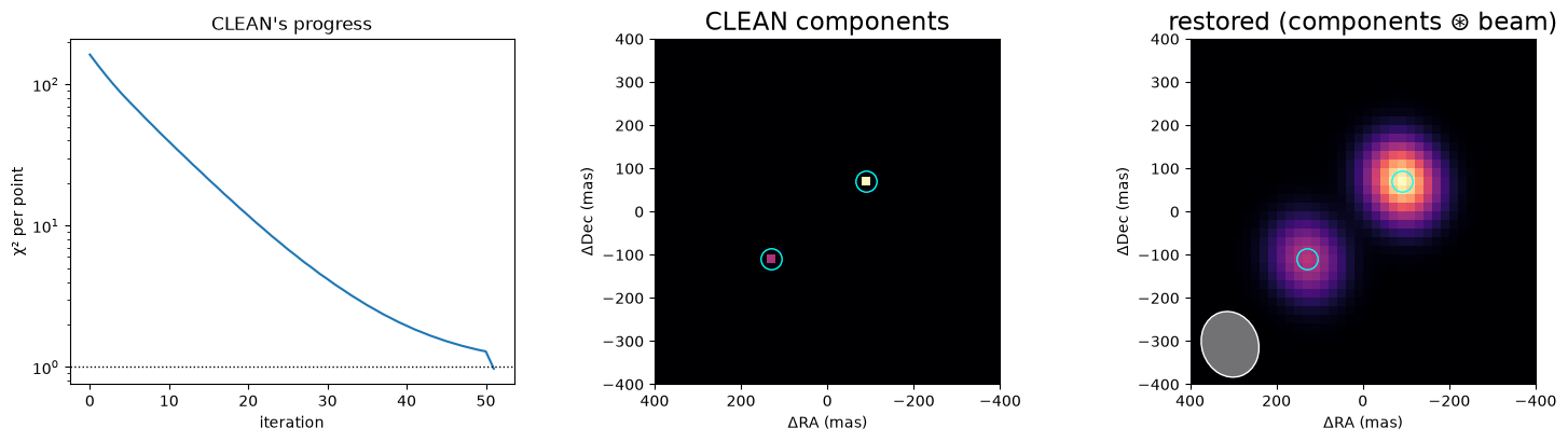
χ² per point falls steadily from about 160 to 1.3 over the first 50 iterations. Then the first major cycle refits the components' fluxes, and takes χ² straight to the target. After it, the flux sits on the companion and the knot (circled), with only faint components on the pixels next to them. The restored image, the components convolved with the beam, is the radio astronomers' way of showing what the data resolve; virgil's plot_model(..., beam=, convolve=True) draws it.
fig, axes = plt.subplots(1, 3, figsize=(15, 4.2))
axes[0].semilogy(result.chi2_red)
axes[0].axhline(1.0, color="k", ls=":", lw=1)
axes[0].set(xlabel="iteration", ylabel="χ² per point", title="CLEAN's progress")
plot_model(result.model.clean, fov, npix, ax=axes[1], title="CLEAN components")
plot_model(
    result.model.clean, fov, npix, ax=axes[2], beam=resolution, convolve=True,
    title="restored (components ⊛ beam)",
)
for ax in axes[1:]:
    ax.plot([-90, 130], [70, -110], "o", mfc="none", mec="cyan", ms=14)
plt.tight_layout()
plt.show()
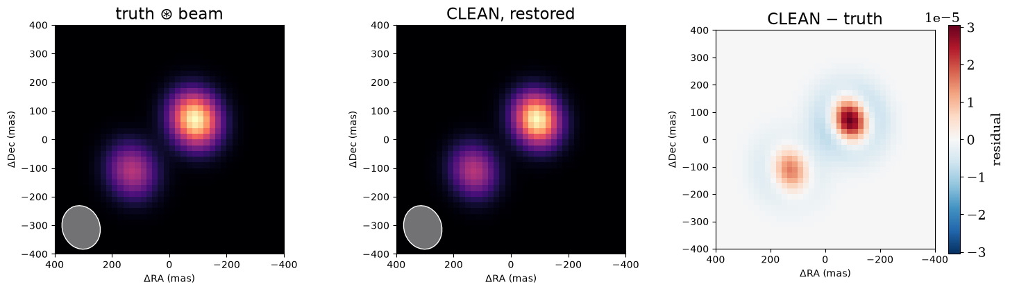
How close is the restored image to the truth? Here both are convolved with the beam and scaled to their total fluxes, relative to the star, and the right panel is their signed difference. The CLEAN image is a point estimate with no uncertainties, so these are plain differences, not z-scores. They peak at about 10% of the brightest pixel of the truth, positive at both sources with a faint negative ring around them: CLEAN's sources come out a little more compact than the truth as drawn on this grid. Their fluxes are, if anything, slightly low (0.0194 and 0.0092 against 0.02 and 0.01).
# render() gives unit-flux images: scale each by its flux relative to the star.
truth_smooth = 0.03 * convolve_beam(faint.render(npix, fov), scale, resolution)
clean_smooth = float(components.sum()) * convolve_beam(
    result.model.clean.render(npix, fov), scale, resolution
)
fig, axes = plt.subplots(1, 3, figsize=(15, 4.3))
plot_model(faint, fov, npix, ax=axes[0], beam=resolution, convolve=True, title="truth ⊛ beam")
plot_model(
    result.model.clean, fov, npix, ax=axes[1], beam=resolution, convolve=True,
    title="CLEAN, restored",
)
plot_residual_map(clean_smooth - truth_smooth, fov, ax=axes[2], title="CLEAN − truth")
plt.tight_layout()
plt.show()
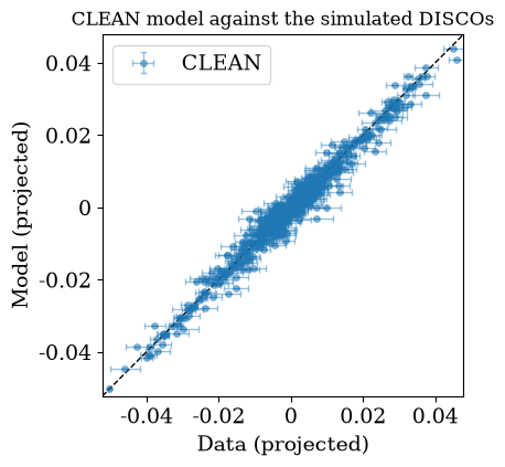
An image that looks right should also fit the data. The correlation plot compares the CLEAN model's predictions with the data, with the data's error bars and a one-to-one line. AMI DISCO observables are projections that mix amplitude and phase information, so they appear in a single panel. The points scatter evenly about the line across the full range: the components explain the data.
n_vis = data.vis.size
prediction = data.model(result.model)
summary = {
    "CLEAN": {
        "vis_mean": prediction[:n_vis],
        "vis_std": 0 * prediction[:n_vis],
        "phi_mean": prediction[n_vis:],
        "phi_std": 0 * prediction[n_vis:],
    }
}
fig, (ax, _) = plot_data_model_correlation(data, summary, figsize=(5, 4.5))
ax.set_title("CLEAN model against the simulated DISCOs")
plt.show()
Refining the fluxes
The major cycles already refit the components' fluxes inside CLEAN, but only every 50 iterations, and only those fluxes. Because the model is a System with an Image, fit can do the same job on the components' support, and free other parameters alongside them, such as the components' spectrum or the base's fluxes. It is a small, well-posed problem: a few pixels, not the whole grid, so it needs no regulariser. Here, with the fluxes already refitted by the major cycle, it changes nothing.
priors = image_priors(result.model) | {"clean.flux": dist.LogUniform(1e-3, 1.0)}
polished = fit(result.model, priors, data)
print(
    f"flux {float(components.sum()):.4f} after CLEAN, "
    f"{float(polished.model.clean.flux):.4f} refitted (truth 0.030); "
    f"χ²/N {polished.info['chi2_red']:.3f}"
)
flux 0.0297 after CLEAN, 0.0297 refitted (truth 0.030); χ²/N 0.975
The loop gain
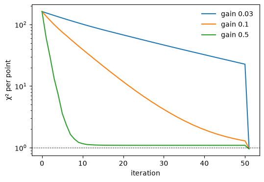
The loop gain trades speed against care. A small gain takes many small steps, and can correct an early step with later ones. A large gain moves quickly, but a step that overshoots cannot be undone, because clean only ever adds flux (so the image stays positive). The major cycles remove that limitation. Here a gain of 0.5 gets χ² per point to about 1.1 within ten iterations and then stalls, because its early steps put flux in the wrong places. The first major cycle, at iteration 50, moves that flux and reaches the target; without major cycles (refit_every=0) CLEAN would stop there, stalled. A gain of 0.03 is still at χ² per point of about 20 after 50 iterations, but by then it has found the right three pixels, and the major cycle solves for their fluxes. All three gains end at the target after the same major cycle, with 3, 6 and 13 components: the larger the gain, the more stray components it leaves. Values of 0.05–0.2 are still the usual choice.
fig, ax = plt.subplots(figsize=(6, 4))
for gain in (0.03, 0.1, 0.5):
    run = clean(data, npix, scale, base=PointSource(), support=support, gain=gain)
    print(
        f"gain {gain}: {len(run.chi2_red) - 1} iterations, "
        f"{int((run.components > 0).sum())} components, flux "
        f"{float(run.components.sum()):.4f}, stopped ({run.stop})"
    )
    ax.semilogy(run.chi2_red, label=f"gain {gain}")
ax.axhline(1.0, color="k", ls=":", lw=1)
ax.set(xlabel="iteration", ylabel="χ² per point")
ax.legend(frameon=False)
plt.show()
gain 0.03: 51 iterations, 3 components, flux 0.0297, stopped (target)
gain 0.1: 51 iterations, 6 components, flux 0.0297, stopped (target)
gain 0.5: 51 iterations, 13 components, flux 0.0302, stopped (target)
Closure phases and V² from a long-baseline interferometer
Classic CLEAN needs Fourier phases; with closure phases it has to be wrapped in self-calibration loops. Gradient CLEAN does not: it fits closure phases and squared visibilities directly, through the same likelihood as fit.
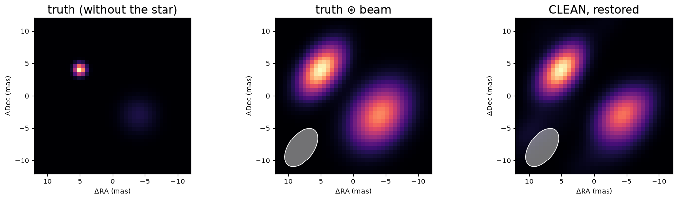
Here are four VLTI unit telescopes in the L band, at five hour angles, with a star, a 3% companion and a 4% extended blob. The blob is larger than the beam, so CLEAN builds it from a cluster of components. CLEAN stops after the first major cycle, at χ² per point of 0.92, with 97% of the true flux; the restored image matches the truth convolved with the beam, including the beam's elongation.
vlti = vlti_oidata()
vfov, vnpix = field_of_view(vlti), 40
vscale = vfov / vnpix
blob = gaussian_blob(vnpix, vscale, 2.0, dra=-4.0, ddec=-3.0)
vtruth = System(
    star=PointSource(),
    companion=PointSource(dra=5.0, ddec=4.0, flux=0.03),
    blob=Image.from_brightness(blob, vscale, flux=0.04),
)
vdata = vlti.with_model(vtruth, key=jax.random.PRNGKey(1))
vbeam = beam(vdata)
vsupport = circular_support(
    vnpix, vscale, radius_mas=vfov / 2, inner_radius_mas=0.5 * vbeam.minor_mas
)
vresult = clean(vdata, vnpix, vscale, base=PointSource(), support=vsupport)
print(
    f"{vdata.vis.size} V² and {vdata.phi.size} closure phases; field "
    f"{vfov:.1f} mas, beam {vbeam.major_mas:.1f} × {vbeam.minor_mas:.1f} mas"
)
print(
    f"stopped ({vresult.stop}) after {len(vresult.chi2_red) - 1} iterations at "
    f"χ²/N = {float(vresult.chi2_red[-1]):.3f}: {int((vresult.components > 0).sum())} "
    f"components with flux {float(vresult.components.sum()):.4f} (truth 0.070)"
)

envelope = System(
    companion=PointSource(dra=5.0, ddec=4.0, flux=0.03),
    blob=Image.from_brightness(blob, vscale, flux=0.04),
)
fig, axes = plt.subplots(1, 3, figsize=(15, 4.2))
plot_model(envelope, vfov, vnpix, ax=axes[0], title="truth (without the star)")
plot_model(
    envelope, vfov, vnpix, ax=axes[1], beam=vbeam, convolve=True,
    title="truth ⊛ beam",
)
plot_model(
    vresult.model.clean, vfov, vnpix, ax=axes[2], beam=vbeam, convolve=True,
    title="CLEAN, restored",
)
plt.tight_layout()
plt.show()
330 V² and 220 closure phases; field 24.1 mas, beam 6.8 × 3.9 mas
stopped (target) after 51 iterations at χ²/N = 0.921: 17 components with flux 0.0677 (truth 0.070)
Summary
cleanbuilds an image from point components where they lower χ² most. It works for any data virgil fits: DISCOs, kernel and closure phases, V², or a mix.- Give it a fixed
base(usually the star), asupportwith a hole under the star, and trust its stopping rule only as far as you trust the error bars. - The result is an ordinary model. Refit its fluxes with
fiton the components' support, show it restored with the beam, or use it as the starting image of a regularised fit. - Each iteration only adds flux; the major cycles move it between components and remove those left with none, so an early mistake no longer stays. CLEAN stops by itself when χ² stalls. The base scene is fixed, and the components share one spectrum: grey by default, or
spectrum=for SPARCO-style imaging. - For extended emission, a regularised fit started from the CLEAN image usually does better.
notebooks/mwe/mwe_sparse_imaging.ipynbcompares CLEAN with the sparsity regularisersStarletL1andLogSumand with maximum entropy, each started from CLEAN.