Visibility Models

This tutorial explains how BinaryModelCartesian and BinaryModelAngular work internally, how they interact with OIData, and how likelihoods are built from an OIData instance plus a model class.

Introduce the visibility model parameterizations

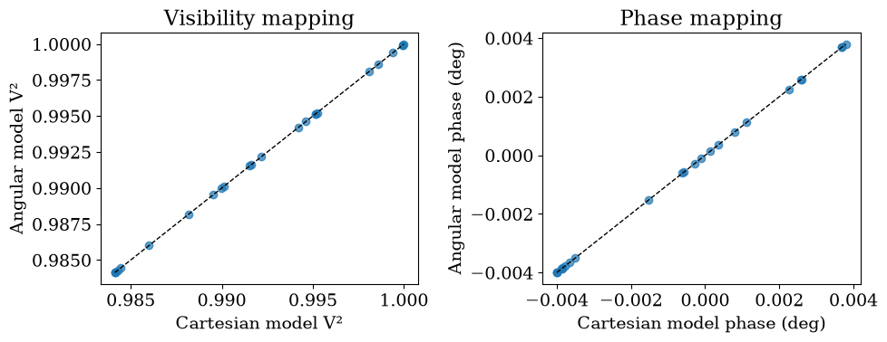
We first define the Cartesian and angular binary models on the same baseline geometry, and verify they produce equivalent complex visibilities when parameters are converted consistently.

import sys
from pathlib import Path

import numpy as np
import jax.numpy as jnp
import matplotlib.pyplot as plt

from virgil.plotting import set_style

repo_root = Path.cwd()
if not (repo_root / "src").exists():
    repo_root = repo_root.parent
src_path = repo_root / "src"
if str(src_path) not in sys.path:
    sys.path.insert(0, str(src_path))

from virgil.likelihood import loglike
from virgil.limits import flux_to_contrast, flux_to_delta_mag
from virgil.models import BinaryModelAngular, BinaryModelCartesian
from virgil.oidata import OIData

set_style()  # the figure style used throughout the docs

Generate OIData from models

Now we generate synthetic observables from the Cartesian model and package them into an OIData instance.

These models are parametrized functions that take a set of parameters like sep, pa and flux, and instantiate an object - say, model - which can then apply these to data. You then call model.model(u, v, wavel) and it evaluates the complex visibilities at those coordinates.

rng = np.random.default_rng(21)
u = jnp.array(rng.uniform(-30.0, 30.0, size=24))
v = jnp.array(rng.uniform(-30.0, 30.0, size=24))
wavel = jnp.array([4.8e-6])

truth_cart = {"dra": 120.0, "ddec": -80.0, "flux": 4e-3}
model_cart_true = BinaryModelCartesian(**truth_cart)

dra = float(truth_cart["dra"])
ddec = float(truth_cart["ddec"])
flux = float(truth_cart["flux"])
sep = float(np.sqrt(dra**2 + ddec**2))
pa = float((np.degrees(np.arctan2(dra, ddec)) + 360.0) % 360.0)
model_ang = BinaryModelAngular(sep=sep, pa=pa, flux=flux)

cvis_true = model_cart_true.model(u, v, wavel)
cvis_ang = model_ang.model(u, v, wavel)
max_complex_diff = float(np.max(np.abs(np.asarray(cvis_ang - cvis_true))))

{
    "cartesian": truth_cart,
    "angular": {"sep": sep, "pa": pa, "flux": flux},
    "max_complex_visibility_difference": max_complex_diff,
}

{'cartesian': {'dra': 120.0, 'ddec': -80.0, 'flux': 0.004},
 'angular': {'sep': 144.22205101855957,
  'pa': 123.69006752597977,
  'flux': 0.004},
 'max_complex_visibility_difference': 3.7834979593753815e-09}

OIData stores observables, uncertainties, and convention flags (v2_flag and cp_flag) so model outputs can be converted and flattened consistently. It flattens all these data into vectors and keeps track of what kind of observable is being used.

vis_true = jnp.abs(cvis_true) ** 2
phi_true = jnp.rad2deg(jnp.angle(cvis_true))

d_vis = (
    0.002 * jnp.maximum(jnp.median(vis_true), 1e-6) * jnp.ones_like(vis_true)
)
d_phi = (
    0.01
    * jnp.maximum(jnp.median(jnp.abs(phi_true)), 5.0)
    * jnp.ones_like(phi_true)
)

vis_obs = vis_true + d_vis * jnp.array(rng.normal(size=vis_true.shape))
phi_obs = phi_true + d_phi * jnp.array(rng.normal(size=phi_true.shape))

data = OIData(
    {
        "u": u,
        "v": v,
        "wavel": wavel,
        "vis": vis_obs,
        "d_vis": d_vis,
        "phi": phi_obs,
        "d_phi": d_phi,
        "phi_unit": "deg",
        "i_cps1": None,
        "i_cps2": None,
        "i_cps3": None,
        "v2_flag": True,
        "cp_flag": False,
    }
)

{
    "n_baselines": int(data.u.shape[0]),
    "v2_flag": bool(data.v2_flag),
    "cp_flag": bool(data.cp_flag),
}

{'n_baselines': 24, 'v2_flag': True, 'cp_flag': False}

How `OIData.model(...)` builds comparable vectors

OIData.model(model) evaluates complex visibilities through the model and converts them to the configured observables (V² and phases here), then flattens to match OIData.flatten_data().

model_vector = data.model(model_cart_true)
data_vector, err_vector = data.flatten_data()

{
    "model_len": int(model_vector.shape[0]),
    "data_len": int(data_vector.shape[0]),
    "error_len": int(err_vector.shape[0]),
    "vector_alignment": bool(
        model_vector.shape == data_vector.shape == err_vector.shape
    ),
}

{'model_len': 48, 'data_len': 48, 'error_len': 48, 'vector_alignment': True}

Cartesian vs angular parameter conversions

The Cartesian model uses \((\Delta\mathrm{RA},\Delta\mathrm{Dec}, f)\), where \(f\) is the companion/primary flux ratio. The angular model uses \((\rho,\mathrm{PA}, f)\) with the same flux ratio. The conversion is:

\[ \rho = \sqrt{\Delta\mathrm{RA}^2 + \Delta\mathrm{Dec}^2}, \quad \mathrm{PA} = \mathrm{atan2}(\Delta\mathrm{RA}, \Delta\mathrm{Dec}) \]

Results are usually reported as a contrast \(C = 1/f\) (primary/companion) or \(\Delta m = 2.5 \log_{10} C\): a companion 100 times fainter has \(f = 0.01\), \(C = 100\) and \(\Delta m = 5\) mag. virgil.limits.flux_to_contrast and flux_to_delta_mag do the conversion.

dra = float(truth_cart["dra"])
ddec = float(truth_cart["ddec"])
flux = float(truth_cart["flux"])

sep = float(np.sqrt(dra**2 + ddec**2))
pa = float((np.degrees(np.arctan2(dra, ddec)) + 360.0) % 360.0)
model_ang = BinaryModelAngular(sep=sep, pa=pa, flux=flux)
cvis_ang = model_ang.model(u, v, wavel)
max_complex_diff = float(np.max(np.abs(np.asarray(cvis_ang - cvis_true))))

{
    "sep_mas": sep,
    "pa_deg": pa,
    "flux": flux,
    # Reported the astronomical way: primary/companion, and in magnitudes.
    "contrast": float(flux_to_contrast(flux)),
    "delta_mag": float(flux_to_delta_mag(flux)),
    "max_complex_visibility_difference": max_complex_diff,
}

{'sep_mas': 144.22205101855957,
 'pa_deg': 123.69006752597977,
 'flux': 0.004,
 'contrast': 250.0,
 'delta_mag': 5.994850021680094,
 'max_complex_visibility_difference': 3.7834979593753815e-09}

vis_cart = np.asarray(data.to_vis(cvis_true))
vis_ang = np.asarray(data.to_vis(cvis_ang))
phi_cart = np.asarray(data.to_phases(cvis_true))
phi_ang = np.asarray(data.to_phases(cvis_ang))

fig, (ax1, ax2) = plt.subplots(1, 2, figsize=(10, 4))

ax1.scatter(vis_cart, vis_ang, alpha=0.7)
line_v = np.linspace(
    min(vis_cart.min(), vis_ang.min()), max(vis_cart.max(), vis_ang.max()), 100
)
ax1.plot(line_v, line_v, "k--", lw=1)
ax1.set_xlabel("Cartesian model V²")
ax1.set_ylabel("Angular model V²")
ax1.set_title("Visibility mapping")

ax2.scatter(phi_cart, phi_ang, alpha=0.7)
line_p = np.linspace(
    min(phi_cart.min(), phi_ang.min()), max(phi_cart.max(), phi_ang.max()), 100
)
ax2.plot(line_p, line_p, "k--", lw=1)
ax2.set_xlabel("Cartesian model phase (deg)")
ax2.set_ylabel("Angular model phase (deg)")
ax2.set_title("Phase mapping")

plt.tight_layout()
plt.show()

model_syntax output 12.1

Likelihood wiring from `OIData` + model class

loglike(values, params, model, data) zips parameter names to values, instantiates model(**param_dict) (or, for a template model instance, sets the leaves at those paths), evaluates data.model(...), then compares to flattened data with Gaussian errors.

params_cart = ["dra", "ddec", "flux"]
vals_cart = [dra, ddec, flux]
ll_cart = float(loglike(vals_cart, params_cart, BinaryModelCartesian, data))

params_ang = ["sep", "pa", "flux"]
vals_ang = [sep, pa, flux]
ll_ang = float(loglike(vals_ang, params_ang, BinaryModelAngular, data))

ll_cart_perturbed = float(
    loglike(
        [dra + 20.0, ddec - 20.0, flux * 1.6],
        params_cart,
        BinaryModelCartesian,
        data,
    )
)

{
    "ll_cart_true": ll_cart,
    "ll_ang_equivalent": ll_ang,
    "ll_cart_perturbed": ll_cart_perturbed,
    "true_beats_perturbed": bool(ll_cart > ll_cart_perturbed),
}

{'ll_cart_true': 259.32464599609375,
 'll_ang_equivalent': 259.32464599609375,
 'll_cart_perturbed': -580.6997680664062,
 'true_beats_perturbed': True}

This gives a practical under-the-hood view: model classes define parameter syntax and complex visibilities, OIData defines observable conventions and flattening, and loglike stitches both pieces together for inference workflows.