Extended source models
This tutorial mirrors the binary-model walkthrough style, but focuses on the non-binary source models in virgil: a star plus a GaussianDisk, the UniformDisk and ModulatedGaussianRim building blocks, and GravityDarkenedStar (a rapidly rotating star). Spotted stars from harmonix, wrapped in HarmonixModel, have their own tutorial.
We'll build synthetic interferometric observables from a resolved Gaussian disk, pass them through OIData, then do the same for a uniform disk and an azimuthally modulated rim, and finally draw a gravity-darkened rapid rotator. See the composition tutorial for how to combine these building blocks into more complex scenes.
import sys
from pathlib import Path

import numpy as np
import jax.numpy as jnp
import matplotlib.pyplot as plt

from virgil.plotting import set_style

repo_root = Path.cwd()
if not (repo_root / "src").exists():
    repo_root = repo_root.parent
src_path = repo_root / "src"
if str(src_path) not in sys.path:
    sys.path.insert(0, str(src_path))

from virgil.models import (
    GaussianDisk,
    ModulatedGaussianRim,
    PointSource,
    System,
    UniformDisk,
)
from virgil.oidata import OIData

set_style()  # the figure style used throughout the docs
Simulate resolved-disk observables
As with the binary examples, we start from a simple baseline geometry, instantiate a source model, and evaluate complex visibilities on those baselines.
rng = np.random.default_rng(7)
n_bl = 32
u = jnp.array(rng.uniform(-24.0, 24.0, size=n_bl))
v = jnp.array(rng.uniform(-24.0, 24.0, size=n_bl))
wavel = jnp.full((n_bl,), 1.65e-6)

truth = {"sigma": 18.0, "flux": 0.15, "dra": 12.0, "ddec": -7.5}
disk = System(star=PointSource(), disk=GaussianDisk(**truth))
cvis_true = disk.model(u, v, wavel)

vis_true = jnp.abs(cvis_true) ** 2
phi_true = jnp.rad2deg(jnp.angle(cvis_true))

vis_scale = jnp.maximum(jnp.median(vis_true), 1e-6)
phi_scale = jnp.maximum(jnp.median(jnp.abs(phi_true)), 5.0)
d_vis = 0.01 * vis_scale * jnp.ones_like(vis_true)
d_phi = 0.02 * phi_scale * jnp.ones_like(phi_true)

vis_obs = vis_true + d_vis * jnp.array(rng.normal(size=vis_true.shape))
phi_obs = phi_true + d_phi * jnp.array(rng.normal(size=phi_true.shape))

data = OIData({
    "u": u,
    "v": v,
    "wavel": wavel,
    "vis": vis_obs,
    "d_vis": d_vis,
    "phi": phi_obs,
    "d_phi": d_phi,
    "i_cps1": None,
    "i_cps2": None,
    "i_cps3": None,
    "v2_flag": True,
    "cp_flag": False,
})

{
    "n_baselines": int(n_bl),
    "sigma_mas": truth["sigma"],
    "flux": truth["flux"],
    "centroid_mas": (truth["dra"], truth["ddec"]),
    "vis_range": (float(jnp.min(vis_true)), float(jnp.max(vis_true))),
}
{'n_baselines': 32,
 'sigma_mas': 18.0,
 'flux': 0.15,
 'centroid_mas': (12.0, -7.5),
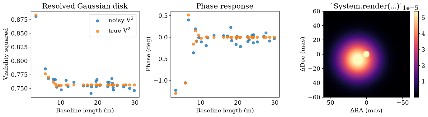
 'vis_range': (0.7543692588806152, 0.8830579519271851)}
Use OIData to flatten observables
OIData.model(...) evaluates the source model, converts complex visibilities to the configured observables, and flattens the result into a vector that can be compared directly to the measured data.
model_vec = data.model(disk)
data_vec, err_vec = data.flatten_data()

{
    "model_len": int(model_vec.shape[0]),
    "data_len": int(data_vec.shape[0]),
    "error_len": int(err_vec.shape[0]),
    "vector_alignment": bool(
        model_vec.shape == data_vec.shape == err_vec.shape
    ),
}
{'model_len': 64, 'data_len': 64, 'error_len': 64, 'vector_alignment': True}
Visualize the Gaussian disk in Fourier and image space
A resolved Gaussian disk has visibility amplitudes that fall smoothly with baseline length. The new render(...) method gives a matching image-plane representation for plotting and sanity checks.
baseline = np.sqrt(np.asarray(u) ** 2 + np.asarray(v) ** 2)
image = np.asarray(disk.render(npix=128, fov_mas=120.0))

fig, axes = plt.subplots(1, 3, figsize=(14, 4))

axes[0].scatter(baseline, np.asarray(vis_obs), alpha=0.8, label="noisy V$^2$")
axes[0].scatter(baseline, np.asarray(vis_true), alpha=0.8, label="true V$^2$")
axes[0].set_xlabel("Baseline length (m)")
axes[0].set_ylabel("Visibility squared")
axes[0].set_title("Resolved Gaussian disk")
axes[0].legend(loc="best")

axes[1].scatter(baseline, np.asarray(phi_obs), alpha=0.8, label="noisy phase")
axes[1].scatter(baseline, np.asarray(phi_true), alpha=0.8, label="true phase")
axes[1].set_xlabel("Baseline length (m)")
axes[1].set_ylabel("Phase (deg)")
axes[1].set_title("Phase response")

im = axes[2].imshow(
    image,
    extent=[60.0, -60.0, -60.0, 60.0],
    cmap="magma",
    vmax=np.quantile(image, 0.99),  # saturate the unresolved star
)
axes[2].set_xlabel(r"$\Delta$RA (mas)")
axes[2].set_ylabel(r"$\Delta$Dec (mas)")
axes[2].set_title("`System.render(...)`")
fig.colorbar(im, ax=axes[2], fraction=0.046, pad=0.04)

plt.tight_layout()
plt.show()
Spotted stars with harmonix
HarmonixModel wraps a star from harmonix, which computes the visibilities of a spherical-harmonic surface map analytically, so that it simulates, draws and fits like any other virgil model. See Spotted stars with harmonix for a worked example.
Simulate a uniform disk
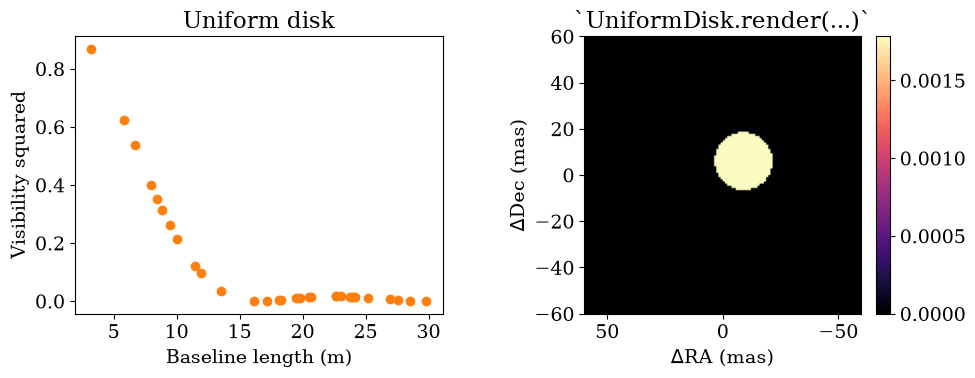
UniformDisk represents a resolved tophat (uniform-brightness) disk. Like every building block it is a pure shape normalized to unit flux; put it in a System with a PointSource if you also want an unresolved star. Its visibility amplitude follows the classic Airy pattern 2*J1(x)/x.
udisk = UniformDisk(diam=25.0, dra=-9.0, ddec=6.0)
cvis_udisk = udisk.model(u, v, wavel)

vis_udisk = jnp.abs(cvis_udisk) ** 2
phi_udisk = jnp.rad2deg(jnp.angle(cvis_udisk))
model_vec_udisk = data.model(udisk)

{
    "diam_mas": float(udisk.diam),
    "centroid_mas": (float(udisk.dra), float(udisk.ddec)),
    "vis_range": (float(jnp.min(vis_udisk)), float(jnp.max(vis_udisk))),
    "model_len": int(model_vec_udisk.shape[0]),
}
{'diam_mas': 25.0,
 'centroid_mas': (-9.0, 6.0),
 'vis_range': (0.0001409070537192747, 0.8681560754776001),
 'model_len': 64}
Visualize the uniform disk in Fourier and image space
Visibility squared falls off with Airy-like nulls as baseline length grows; render(...) gives the matching tophat image.
image_udisk = np.asarray(udisk.render(npix=128, fov_mas=120.0))

fig, axes = plt.subplots(1, 2, figsize=(10, 4))

axes[0].scatter(baseline, np.asarray(vis_udisk), color="tab:orange")
axes[0].set_xlabel("Baseline length (m)")
axes[0].set_ylabel("Visibility squared")
axes[0].set_title("Uniform disk")

im = axes[1].imshow(
    image_udisk,
    extent=[60.0, -60.0, -60.0, 60.0],
    cmap="magma",
)
axes[1].set_xlabel(r"$\Delta$RA (mas)")
axes[1].set_ylabel(r"$\Delta$Dec (mas)")
axes[1].set_title("`UniformDisk.render(...)`")
fig.colorbar(im, ax=axes[1], fraction=0.046, pad=0.04)

plt.tight_layout()
plt.show()
Simulate an azimuthally modulated rim
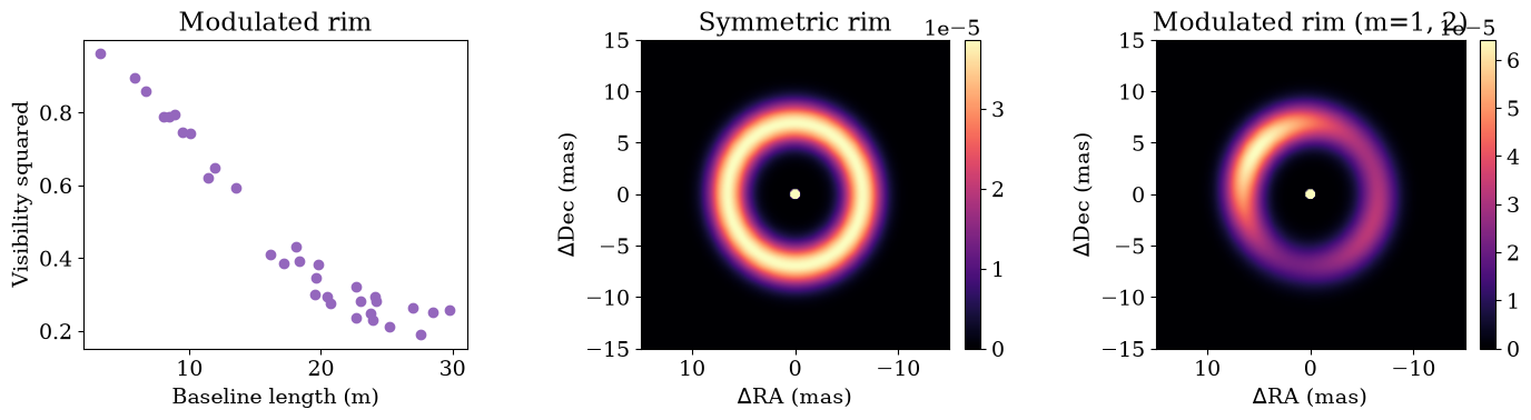
ModulatedGaussianRim is an inclined, Gaussian-blurred ring, optionally modulated azimuthally with a sum of cosine terms (az_amps/az_pas). Adding a PointSource puts an unresolved star at the centre; the rim's flux is then its flux relative to the star. We compare a symmetric rim against one with first- and second-order modulations.
rim_geometry = dict(diam=14.15, fwhm=3.233, inc=19.0, pa=6.0, flux=0.67504187604)
rim = ModulatedGaussianRim(
    **rim_geometry,
    az_amps=jnp.array([0.43011627, 0.2745906]),
    az_pas=jnp.array([35.537678 + 6.0, 50.245735 + 6.0]),
)
rim_symmetric = System(star=PointSource(), rim=ModulatedGaussianRim(**rim_geometry))
rim_modulated = System(star=PointSource(), rim=rim)

cvis_rim = rim_modulated.model(u, v, wavel)
vis_rim = jnp.abs(cvis_rim) ** 2
phi_rim = jnp.rad2deg(jnp.angle(cvis_rim))
model_vec_rim = data.model(rim_modulated)

{
    "diam_mas": float(rim.diam),
    "rim_to_star_flux": float(rim.flux),
    "az_amps": np.asarray(rim.az_amps).tolist(),
    "az_pas_deg": np.asarray(rim.az_pas).tolist(),
    "model_len": int(model_vec_rim.shape[0]),
}
{'diam_mas': 14.149999618530273,
 'rim_to_star_flux': 0.6750418543815613,
 'az_amps': [0.4301162660121918, 0.2745906114578247],
 'az_pas_deg': [41.53767776489258, 56.24573516845703],
 'model_len': 64}
Visualize the rim: azimuthal modulation and Fourier response
Rendering both variants side by side shows how az_amps/az_pas breaks the ring's azimuthal symmetry; the visibility-squared panel shows the modulated rim's (flux-mixed) Fourier response. The parameters are chosen here so the modulated rim model and its image
match the final geometric model shown for the post-AGB IRAS 08544-4431 in Hillen et al. 2016.
image_rim_symmetric = np.asarray(rim_symmetric.render(npix=256, fov_mas=30.0))
image_rim_modulated = np.asarray(rim_modulated.render(npix=256, fov_mas=30.0))

fig, axes = plt.subplots(1, 3, figsize=(14, 4))

axes[0].scatter(baseline, np.asarray(vis_rim), color="tab:purple")
axes[0].set_xlabel("Baseline length (m)")
axes[0].set_ylabel("Visibility squared")
axes[0].set_title("Modulated rim")

im1 = axes[1].imshow(
    image_rim_symmetric,
    extent=[15.0, -15.0, -15.0, 15.0],
    cmap="magma",
    vmax=np.quantile(image_rim_symmetric, 0.999),  # saturate the unresolved star
)
axes[1].set_xlabel(r"$\Delta$RA (mas)")
axes[1].set_ylabel(r"$\Delta$Dec (mas)")
axes[1].set_title("Symmetric rim")
fig.colorbar(im1, ax=axes[1], fraction=0.046, pad=0.04)

im2 = axes[2].imshow(
    image_rim_modulated,
    extent=[15.0, -15.0, -15.0, 15.0],
    cmap="magma",
    vmax=np.quantile(image_rim_modulated, 0.999),
)
axes[2].set_xlabel(r"$\Delta$RA (mas)")
axes[2].set_ylabel(r"$\Delta$Dec (mas)")
axes[2].set_title("Modulated rim (m=1, 2)")
fig.colorbar(im2, ax=axes[2], fraction=0.046, pad=0.04)

plt.tight_layout()
plt.show()
A rapidly rotating star: GravityDarkenedStar
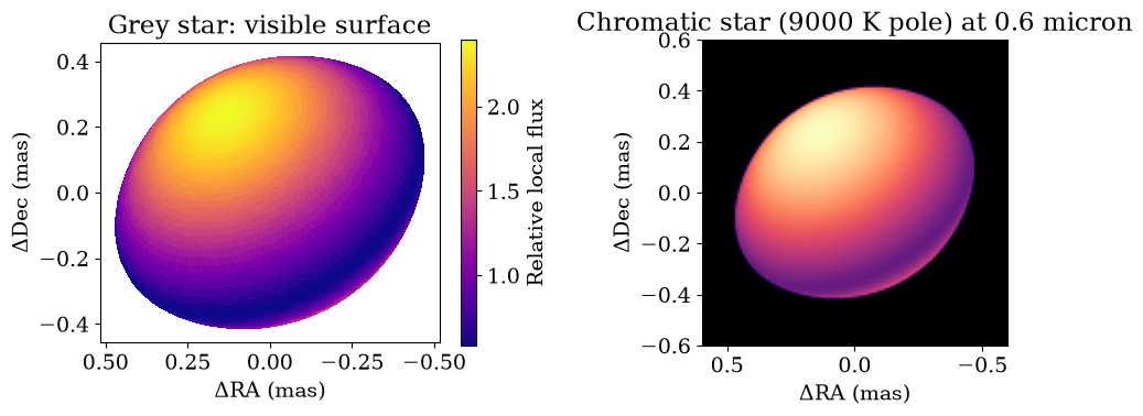
GravityDarkenedStar models a star spinning close to break-up, using the Roche shape and gravity darkening of Espinosa Lara & Rieutord (2011), which needs no free gravity-darkening exponent. The model is Shashank Dholakia's port of ELR11 into JAX (from his jax-interferometry code), brought into virgil with his ELR_Model as its grey mode. Its parameters are the equatorial angular diameter diam_eq in mas, the rotation rate omega as a fraction of the critical rate (0 is a sphere), the inclination inc in degrees (0 is pole-on, 90 equator-on), and pa, the position angle of the visible rotation pole, North through East. The mesh resolution is set by n_lat.
By default the star is grey: its brightness pattern is the same at every wavelength. Passing t_pole, the pole's effective temperature in kelvin, switches on a chromatic mode in which each patch of the surface radiates as a black body, so the contrast between the hot pole and the cool equator grows towards short wavelengths; wavel0 is the wavelength at which render draws it. Like the other components it can be placed in a System, for example with a companion. See the MWE notebook for a fit to simulated multi-channel VLTI data.
from virgil.models import GravityDarkenedStar

star = GravityDarkenedStar(1.0, omega=0.9, inc=50.0, pa=30.0, n_lat=64)
hot_star = GravityDarkenedStar(
    1.0, omega=0.9, inc=50.0, pa=30.0, n_lat=64, t_pole=9000.0, wavel0=0.6e-6
)
cvis_star = star.model(u, v, wavel)

{
    "diam_eq_mas": float(star.diam_eq),
    "omega": float(star.omega),
    "n_baselines": int(cvis_star.shape[0]),
    "vis_range": (
        float(jnp.min(jnp.abs(cvis_star) ** 2)),
        float(jnp.max(jnp.abs(cvis_star) ** 2)),
    ),
}
{'diam_eq_mas': 1.0,
 'omega': 0.8999999761581421,
 'n_baselines': 32,
 'vis_range': (0.9856705069541931, 0.9998699426651001)}
The grey star's visible surface, coloured by local flux, shows the bright pole towards the upper left (with East to the left and North up, the pole at a position angle of 30 degrees) and the darkened equator. The chromatic star at 0.6 micron, drawn through render, is the same shape with the equator much dimmer than the pole.
from virgil.plotting import plot_model

fig, axes = plt.subplots(1, 2, figsize=(10, 4))

star.plot_surface(ax=axes[0])
axes[0].set_title("Grey star: visible surface")

plot_model(
    hot_star,
    fov_mas=1.2,
    npix=128,
    ax=axes[1],
    title="Chromatic star (9000 K pole) at 0.6 micron",
)

plt.tight_layout()
plt.show()