Radio interferometry
Provisional
May change in any 0.4.x release without a deprecation cycle.
This module is not final and claims no parity with MPoL or with published DSHARP analyses.
virgil.radio fits calibrated complex visibilities at
arbitrary (u, v) points, the data of any radio or millimetre array whose
visibilities are in a CASA measurement set. Any source model works, including a pixel
Image whose Fourier transform runs through
the NUFFT backend. Each observation may have its own flux scale,
phase-centre offset and error scale, fitted together with the sky.
A worked example, on simulated data, is the radio imaging tutorial; CLEAN gives a dirty image and a starting point.
A first fit
Simulate a Gaussian disk at random (u, v) points and fit its width. Real data come from ComplexVisData.read_ms("target.ms").
import numpy as onp
import numpyro.distributions as dist
from virgil import CalibrationNuisance, ComplexVisData, fit
from virgil.models import GaussianDisk

rng = onp.random.default_rng(0)
u, v = rng.uniform(-2e5, 2e5, (2, 2000))             # in wavelengths
lam = 1.3e-3                                           # m; models take metres
vis = onp.asarray(GaussianDisk(300.0).model(u * lam, v * lam, lam))
vis = vis + 0.01 * (rng.normal(size=2000) + 1j * rng.normal(size=2000))
data = ComplexVisData.from_arrays(u, v, vis, 1 / 0.01**2, 230e9)

nuis = CalibrationNuisance(data, alpha=False, offsets=False, sigmas=False)

def scene(values):
    return GaussianDisk(values["sigma"])

def model(**values):
    return scene(values)

priors = nuis.priors() | {"sigma": dist.LogUniform(10.0, 3000.0)}
result = fit(model, priors, (), likelihoods=[data.term(scene, nuis)],
             init=nuis.defaults() | {"sigma": 100.0}, method="lbfgs")
print(result.values["sigma"], result.info["chi2_red"])  # about 300 mas, 1.01
The fit recovers the width, and the raw χ²/N on the quoted errors is 1.01. Here sigmas=False fixes the error scales at 1, so this is the number to quote.
Install
Reading a CASA measurement set needs casatools: pip install "virgil-astro[radio]". ComplexVisData.from_arrays needs nothing extra.
casatools versions
casatools publishes wheels for Python 3.12 and 3.13 in its newest releases
(older releases for 3.11) and none for 3.14, so the extra is skipped on
Python 3.14.
casatools also needs CASA's measures data (see CASA's casaconfig) on
first use.
The extra brings casatools>=6.6. On some systems casatools 6.7.6 fails to
import with a missing OPENSSL_3.0.1 symbol; casatools 6.7.0.31 works
(pip install "casatools==6.7.0.31"). virgil does not pin the version.
Reading data
from virgil import ComplexVisData

data = ComplexVisData.read_ms("target.ms", stride=100)  # every 100th row
read_ms conjugates CASA's DATA column to virgil's convention.
read_ms raises if the selection holds more than one field (a mosaic); pass field= to pick one. It handles one ddid at a time, so memory is that of the largest ddid.
select(ddids=..., obs=...) and subset(mask) keep the labels, so a
calibration model built for the full data still fits.
What read_ms reads, and the sign convention
- The visibility is
V(u, v) = Σ I(x, y) exp(−2πi (u x + v y)), withxtowards East,ytowards North andu,vin wavelengths: virgil's convention everywhere. - The CASA
DATAcolumn is the conjugate of thisV, withu = UVW[0] ν / candv = UVW[1] ν / c.read_msconjugates it for you. This was decided with a point source predicted by CASA's simulator (tests/test_radio.py::test_read_ms_convention, casatools 6.7.6.14): the data match virgil's model to 5×10⁻⁷ with the conjugation and differ by order 1 without it. (The equivalent statement without conjugation isu = −UVW[0] ν / c,v = −UVW[1] ν / c.) - Only cross-correlations are read. A sample is one (row, channel), kept
when the row and both parallel-hand polarizations (XX and YY, or RR and
LL) are unflagged and both weights positive. The two polarizations are
averaged with their weights,
V = (w₁V₁ + w₂V₂)/(w₁ + w₂), with weightw₁ + w₂. - A weight is
1/σ²for each of the real and imaginary parts (CASA's meaning).WEIGHT_SPECTRUMis used if present, otherwiseWEIGHT. obs(OBSERVATION_ID) is relabelled 0..n−1 in sorted order, the originals kept inobs_ids.ddidnumbers the sorted (DATA_DESC_ID, observation) pairs, so a concatenated set in which oneDATA_DESC_IDspans several observations gets a label, and an error scale, for each;ddid_idsholds each label's originalDATA_DESC_ID.
A model with calibration nuisances
The model at a point k of observation e is
M_k = F g_e (ν_k/ν₀)^α exp(−2πi(δα_e u_k + δδ_e v_k)) T(u_k, v_k) V_scene(u_k, v_k)
with the total flux F (Jy), relative gains g_e, phase-centre offsets
(δα_e, δδ_e) in mas, a spectral index α and an optional Gaussian taper
T (a convolution of the image). The reference observation has g = 1 and no
offset. Each ddid label d has an error scale s_d multiplying its errors, fitted
with the Jeffreys prior 1/s (or profiled out, below). The spectral index α has the prior
Uniform(0, 5) by default, which excludes the falling spectra of
synchrotron or free-free sources: pass priors(alpha=(-3, 5)) for those, or
alpha=False to fix it at 0 (or alpha=2.0 at that value). CalibrationNuisance holds this configuration
and the default priors:
import numpy as onp
import numpyro.distributions as dist
from virgil import CalibrationNuisance, Image, fit

nuis = CalibrationNuisance(data, ref_obs=0)  # nu0_hz: the data's mean frequency
priors = nuis.priors()  # cal.flux, cal.gain, cal.offset, cal.sigma, cal.alpha
init = nuis.defaults()

def scene(values):
    return Image(values["log_brightness"], pixel_scale_mas=2.0)

def model(**values):  # the likelihood term holds the data
    return scene(values)

priors["log_brightness"] = dist.Normal(0.0, 3.0)  # per pixel, shape (64, 64)
init["log_brightness"] = onp.zeros((64, 64))     # a flat starting image
term = data.term(scene, nuis, chunk_size=1_000_000)
result = fit(model, priors, data=(), likelihoods=[term], init=init, method="lbfgs")
Vector-valued sites (cal.gain has one entry per non-reference observation) are
ordinary array-valued parameters. Because the error scales are fitted, the
term reports a log normalization and fit uses L-BFGS.
The term evaluates the points in chunks of chunk_size with jax.lax.map,
padded with zero weight, so memory is bounded by the chunk rather than the
number of visibilities.
For a fit with the scene on the model side only, data.model(scene, values,
nuis) returns M_k and data.chi2_by_ddid(scene, values, nuis) the χ² and
number of points of each ddid.
Conditioning
fit optimizes in unconstrained coordinates, and a poorly
scaled coordinate makes L-BFGS crawl. The gains and error scales have the
improper Jeffreys prior 1/x by default (flat in ln x, no box), so the
coordinate is ln x. The offset of observation k is uniform over three
beams (offset_beams=3; one beam is 2π b_k, b_k = 1/(2π q_max,k), q_max,k the
longest baseline of that observation), so a unit step of the coordinate is a few
phase turns at the longest baseline of each observation. An offset known to a
microarcsecond from long baselines and one known to a tenth of a milliarcsecond
from short ones then have curvatures of the same order, where the old
±1/(2 q_min) box (about 10⁴ mas) did not. The bound is a prior: an offset beyond it
is excluded and appears in info["at_bound"], so widen offset_beams if it does.
The site values stay physical (cal.gain, cal.offset in mas, cal.sigma).
Explicit bounds, priors(offset=(lo, hi)) in mas, priors(gain=(0.5, 2)) or
sigma=(0.1, 10), set the scale again.
Loss and profiled error scales
Loss. Per unmasked point the term is ½|r|²/s_d² + 2 ln s_d for
r = (V − M)√w, the two real parts counting as one complex point, so the total
is ½χ² plus log_norm = Σ_k m_k 2 ln s_d(k). The taper is
T = exp(−(πθq)²/(4 ln 2)), θ the FWHM in radians and q = √(u² + v²); the
offset ramp has the sign of a component's dra, ddec.
Profiled error scales. CalibrationNuisance(data, sigmas="profile") has no
cal.sigma site. At every evaluation s_d² = χ²_d(s=1) / (2 N_d), N_d the number
of unmasked complex points of ddid d. The loss of a point is
½|r|²/s² + 2 ln s, and for the Jeffreys prior this s_d is exactly the
maximum over ln s_d, so the profiled optimum of the other parameters is the
joint optimum, found with fewer coordinates and without the degeneracy
between s and the amplitude. The gradient is the partial derivative at ŝ
(the envelope theorem; ŝ is held by stop_gradient). fit returns ŝ in
result.info["derived"]["cal.sigma"] and
data.sigma_hat computes it for any
values. Held-out data are not scored with their own ŝ: pass the training
ŝ as data.term(..., sigma=ŝ), and use sigmas=True with cross_validate. The loss it returns is ½χ²(ŝ) + log_norm(ŝ) = Σ_d N_d (1 + 2 ln ŝ_d), the profile of the joint loss, so losses compare across fits of the same data, profiled or not. The reported χ² is at ŝ (so it is 2 N_d per ddid by construction): quote the
χ² at the quoted errors, Σ_d 2 N_d ŝ_d², instead.
Compiling with the data as arguments
The data live in the term as array leaves, so fit passes them to its jitted
functions as arguments: they are never compile-time constants, and fits that
differ only in the mask (mask=fold != i) or in a regularizer weight reuse one
compiled loss. Keep it that way in your own jitted code by passing the term as
an argument:
import equinox as eqx
import jax.numpy as jnp

@eqx.filter_jit
def loss_and_grad(term, values):
    return eqx.filter_value_and_grad(
        lambda v: 0.5 * jnp.sum(term(v) ** 2) + term.log_norm(v)
    )(values)

loss, grad = loss_and_grad(term, values)
Do not write jax.jit(lambda values: ... term(values) ...): a closure over the
term embeds every visibility in the compiled program (gigabytes at ALMA scale,
with JAX's "large amount of constants were captured" warning, slow compiles and
executables too big for the persistent cache). The same holds for a
jax.jit(jax.value_and_grad(f)) where f closes over term.
Antenna-based gains
Self-calibration solves for the antenna gains and applies them; closure-only
imaging discards them. CalibrationNuisance(data, antenna_gains=True,
solint="scan") instead marginalizes one complex gain
g = exp(λ + iφ) per antenna and solution interval, so the posterior of the
image carries the calibration uncertainty. The model is
V_k = g_i conj(g_j) M_k + noise, with priors λ ~ N(0, τ_a²) and
φ ~ N(0, τ_φ²), independent between antennas and intervals.
solint is "int" (each integration), "scan" or a number of seconds;
intervals never cross a scan. The data need time, ant1 and ant2 (and
scan for "scan"; read_ms fills them).
nuis = CalibrationNuisance(data, antenna_gains=True, solint="scan")
term = data.term(scene, nuis)  # then fit(..., likelihoods=[term], method="lbfgs")
Method
At every evaluation the model M_k is computed once, then a few
(gain_steps, default 5) Gauss–Newton steps from g = 1 give the gain
solution, and the integral over the gains is taken by a Laplace approximation
about it. The Hessian splits into an amplitude block and a phase block
(a weighted graph Laplacian), because the cross terms cancel; each adds
½ log det, from a batched Cholesky factorization. The gradient passes
through the unrolled steps. Centring on the solution, not on g = 1, is what
lets phase errors of about a radian be handled. Larger errors (about two
radians or more) can leave the solution in a local minimum; raise
gain_steps or calibrate first.
The prior widths are choices
cal.gain_amp_width (τ_a, default 0.1) and
cal.gain_phase_width (τ_φ, default 0.5 rad) are not measurements; the
default amplitude width is of the order of ALMA's absolute flux accuracy
(5–20%, by band), and no phase specification exists. Fix them, or fit them
(fit_gain_widths=True: log-uniform priors on 1e-3–10, overridable in
priors; an unbounded 1/τ prior would be improper, since the marginal tends
to a constant as τ → 0).
Caveats
- With
τ → 0the likelihood is the ungained one (up to a constant); withτ → ∞it tends to closure-only inference. The finite phase prior is essential: without it the absolute position is lost, as with closure phases. A snapshot then constrains the source position only throughτ_φ. - The mean
λof an interval is degenerate withcal.fluxandcal.gain; onlyτ_aidentifies it, socal.gainis pinned by the mean over intervals. - Within an interval a per-observation
cal.offsetis a phase gradient that the gains can absorb: with antenna gains it is identified throughτ_φalone. - An amplitude gain rescales the noise too; the model does not know it, so only the phase part of the closure equivalence is exact.
- There is no least-squares form (
fit(method="lm")raisesNoLeastSquaresForm; uselbfgsoradam, ornumpyro_model). Theresidualshold the data and the solved gains over their prior widths, andlog_normthe log-determinants.precondition="diag"sees those rows and omits the log-determinant, so it is approximate. data.modelanddirty_image(scene=...)apply no gains and raise with antenna gains;term.gains(values)returns the solved gains, andchi2_by_ddidis taken at the solution.fit(...).info["derived"]holdscal.gain_step, the size of the last Gauss–Newton step: if it is not small, raisegain_steps.sigmas="profile"takesŝat the gain solution and holds it fixed.- Memory is
n_interval × n_ant²floats per Hessian block; independent intervals only (gains correlated in time are a later stage).
Source: Blackburn et al. (2020), references; Broderick et al. (2020), references; Arras et al. (2019), references.
Blurring kernel: blur_fwhm_mas
Image(..., blur_fwhm_mas=...) and CalibrationNuisance(blur_fwhm_mas=...)
put a fixed Gaussian blurring kernel of that FWHM (mas) in the forward
model: the data are compared with the blurred model, not with a blurred
copy afterwards. The fit then recovers the unblurred sky, and a kernel
wider than the true structure is deconvolved, which can leave dots. The
default is None, which is recommended: fit the underlying image, regularize
it, and blur for display after the reconstruction. (Formerly smooth_fwhm_mas
and taper_fwhm_mas, deprecated aliases until 0.5. This is not CASA's
uvtaper, the data weighting of dirty_image.)
env = Image(eta, 5.0, blur_fwhm_mas=30.0)
reg = MaxEntropy(w, smoothed=True)  # entropy of the blurred image
smoothed=True clips FFT round-off at zero; MaxEntropy and LogSum then
use a flat default over all pixels, since blurring spreads flux beyond the
support. Setting both blurs the model twice, so fit and data.term warn
(UserWarning) when they meet.
What the kernel acts on
CalibrationNuisancemultiplies the visibilities of any scene (a parametric model, anImage, aSystem) byexp(-π² θ² q² / (4 ln 2)). It is a uv-plane factor, so a regularizer, which acts on pixels, never sees it.Imagedeclares that the sky the data see is its pixels convolved with the Gaussian, as in MPoL'sGaussConvFourier(Czekala et al. 2025, references). The visibilities are the same factor times the pixel transform (exact at any uv point for everyft), andImage.smoothed()returns the convolved pixels by an FFT on a zero-padded grid. A regularizer'ssmoothed=Trueoption penalizes those pixels instead of the raw ones; the base image is then unregularized, sofitwarns (UserWarning). MPoL does this; virgil's default does not.
Accuracy
smoothed() crops its result to the image, so flux spreading
past the edges is lost (keep the emission clear of them). For a kernel of at
least 3 pixels FWHM the transform of the smoothed pixels equals the analytic
Gaussian times the raw transform to about exp(-π² θ² (1/p - q)² / (4 ln 2))
of the flux (an upper bound, times the raw transform at the aliased
frequency), p the pixel size: about 1.5e-8 at FWHM 3 px and q = 0.25 / p.
Measured on a compact image in float64 with |q| <= 0.25 / p, the error is
3e-11 of the flux at 3 px. A narrower kernel is not band-limited on the pixel grid, and
the discretization error grows quickly; the visibilities, which use the
analytic factor, stay exact.
Primary beam and cross-validation
primary_beam(npix, pixel_scale_mas, freq_hz, dish_m, factor) is the log
attenuation −4 ln 2 r²/FWHM² of a Gaussian primary beam with
FWHM = factor × λ/dish_m. Nothing is assumed about the telescope: take the
dish diameter and factor from its documentation. For example, ALMA's 12 m
antennas have factor = 1.13 (ALMA Technical Handbook), and ATCA's antennas
are 22 m in diameter (ATNF). Add the result to an Image's log-brightness so
that the image is the sky times the beam.
dartboard_folds(data, k=5) splits the data into k folds for
cross-validation by cells of the uv plane (annuli in q, sectors in the
azimuth mod π), so that a point and its Hermitian partner never straddle a
train/test split and most neighbouring points share a fold (points either
side of a cell edge can still fall in different folds, so scores can be
slightly optimistic). Fit with
term(..., mask=fold != i) and score the held-out points with
chi2_by_ddid(..., mask=fold == i).
Toeplitz χ²
A worked example, on simulated data, is the radio imaging tutorial.
fit picks this form itself (ComplexVisData.term(..., chi2="auto")) when it
is exact: one fixed Image, offsets=False, a fixed alpha, no
antenna_gains, float64, method="lbfgs" or "adam", and enough points per pixel
and ddid (set_ft_defaults; about 24 N² bytes of device memory per ddid, capped by toeplitz_max_bytes; fit(...).info["likelihood_forms"] says what ran). Otherwise it stays direct; chi2="toeplitz" demands it
and chi2="direct" forbids it. numpyro_model and the fits of cross_validate are always
direct. Build it by hand, as below, for fitted offsets.
Precompute the dirty image and the dirty beam once, and an evaluation costs a few FFTs of the image, whatever the number of visibilities:
import jax

jax.config.update("jax_enable_x64", True)  # float64 is required

nuis = CalibrationNuisance(data, ref_obs=0, alpha=False, offsets=False)  # or alpha=2.0
tdata = data.toeplitz(Image(init["log_brightness"], pixel_scale_mas=2.0), nuis)
term = tdata.term(scene, nuis)
result = fit(model, priors, data=(), likelihoods=[term], init=init,
             method="lbfgs", precondition="diag")
The term has the loss, gradient, profiled ŝ and info["derived"] of
data.term(scene, nuis) for the same points, but no residual vector: fit
with "lbfgs" or "adam" ("lm", gauss_newton_mass and the Gauss–Newton
covariance raise NoLeastSquaresForm). With precondition="diag" the pixel,
flux and gain diagonal is the exact Gauss–Newton one of the direct term; the
offsets and error scales take the diagonal of the loss Hessian.
- What it covers. Per-observation gains, the flux, the nuisance blur,
Image(blur_fwhm_mas=...), a mask, and fixed, fitted or profiled error scales. The image layout (shape, pixel scale, rotation, smoothing) is fixed at the precompute; the scene must return that layout, alone or as the only part of aSystem, at the template'sdra,ddec(a fixed shift, folded into the visibilities at the precompute). - What it refuses. A fitted spectral index (pass
alpha=Falseor a number), antenna gains, other components, float32, and fitted offsets unless asked for (below). - Checks.
tdata.crosscheck(scene, values, nuis)compares the χ² per ddid and the loss with the direct term;tdata.direct_term(scene, nuis)is that term. They agree to about 1e-13 of the loss. - New weights.
tdata.rebuild(vis, weight)repeats the precompute for new visibilities or weights without recompiling (bootstraps, reweighting). Weights must stay finite and positive; drop points throughmaskinstead.
The quadratic form
When the scene is one Image, the χ² of each ddid
d (observation e) is a quadratic in the pixels,
χ²_d = (C_d − 2 G_e Iᵀ D_d(δ_e) + G_e² Iᵀ B_d I) / s_d²,
with G_e = F g_e, C_d = Σ w|V|², the dirty image D_d at the
observation's offset δ_e and the dirty beam B_d, a Toeplitz matrix
applied by FFT on a 2N × 2N grid (Fessler et al. 2005).
Fitted offsets (opt-in)
offsets="spread" is an extension. The
offset ramp e^{−2πi u·δ_e} cancels in |M|², so B_d does not depend on
the offsets and only D_d moves. tdata stores each ddid's type-1 spread
grid b (nufftax's exponential-of-semicircle kernel ψ, Barnett et al.
2019), and Poisson summation gives the dirty image at any real position,
D(x + δ) = Σ_l b_l e^{2πil(x+δ)/n_f} / ψ̂(x + δ),
a phase ramp on the stored grid divided by the kernel's transform at a
non-integer position (by quadrature, as in a type-3 NUFFT; Lee & Greengard
2005). It is exact to the kernel tolerance while no point's kernel wraps,
max |t| ≤ π(1 − w/n_f), with t the baseline in radians per pixel. This
builds on type-3 NUFFT evaluation; we know of no prior use of this
combination, so it is opt-in:
nuis = CalibrationNuisance(data, ref_obs=0, alpha=False)  # offsets fitted
tdata = data.toeplitz(template, nuis, offsets="spread")
It refuses baselines past tdata.margin of the pixel Nyquist limit
(tdata.nyquist_fraction is max |t|/π; use smaller pixels or mask the
longest baselines), and offsets beyond the precompute's bound
(max_offset_mas, by default the last nuis.priors(offset=...) bound, so call it first) raise at run time.
Without it, B_d and D_d need only integer lags and are exact at any
baseline.
Performance
No benchmark in the repository reproduces a timing table yet, so none is given. One independent check on a real ALMA data set (virgil-validation, float64, A100 GPU; 42.4 M points, 26 ddids, 1028² pixels of 5 mas, with gain and offset gradients) measured one value-and-gradient evaluation of χ² at 735 ms through the nufftax backend (ft="nufft", eps 1e-6) and 21.8 ms through the Toeplitz path with free offsets (offsets="spread"). The two figures are not shown to share one setup, so their ratio is not a speed-up claim.
Diagnostics
Both diagnostics are model-free displays or checks: neither is part of the likelihood.
Error scale from time-adjacent samples
data.sigma_scale(by="ddid") estimates the error scale s (the factor on the quoted errors 1/√w) without a sky model. It is an upper bound (see the caveats).
res = data.sigma_scale()            # per ddid label; by="obs" or None also work
for label, s, se in zip(res.labels, res.s, res.s_se):
    print(f"ddid {label}: s = {s:.3f} ± {se:.3f}")
How it is estimated
Samples of one baseline,
channel and scan are sorted by time and paired (1st with 2nd, 3rd with
4th, …); a pair has Var(ΔRe) = s²(1/wᵢ + 1/wⱼ), so
ŝ² = mean over pairs of ΔRe² / (1/wᵢ + 1/wⱼ),
the same for Im, and ŝ combines the two. Standard errors are the sample
errors of those means.
Caveats
- It is an upper bound. A change of the sky, gain or phase between the
two integrations adds to
|ΔV|², soŝis biased high where the data vary quickly (atmospheric phase, long integrations). Compare it with the fittedcal.sigma: a fit well belowŝis expected, a fit above it is not. - It needs
time,ant1,ant2andscan, whichread_msfills (otherwisefrom_arrays(..., time=, ant1=, ant2=, scan=)); it raises if they are missing. Withread_ms(stride=k>1)the rows are no longer adjacent. lag_ratiocompares the mean-square difference of far pairs (half a run apart) to adjacent pairs. A ratio well above 1 means the pairing does what it should; near 1 means constant data or a time order that does not follow the data (for example a scrambled time column), so checkŝ.- It sorts one ddid at a time with NumPy and no Python loop over points: memory is a few arrays of the largest ddid's length.
Dirty and residual images
beam = data.dirty_beam(256, 0.5, weighting="briggs", robust=0.5)
dirty = data.dirty_image(256, 0.5, weighting="briggs", robust=0.5)  # Jy/beam
resid = data.dirty_image(
    256, 0.5, weighting="briggs", scene=scene, values=values, nuisance=nuis,
    use_sigma=True,
)  # image of data - model, in Jy/beam
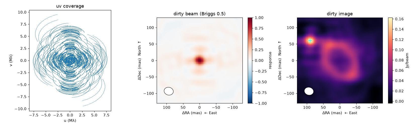
The simulated observation of the CLEAN guide (a ring and a clump, marked +,
North-East of the centre): the uv coverage with its Hermitian mirror, the Briggs dirty beam
and the dirty image, with the beam ellipse in the lower left.
What the image is
The image is Σ wₖ Re[Vₖ e^{+2πi(uₖx + vₖy)}] / Σ wₖ, computed with the
adjoint (type-1) NUFFT of nufftax at the raw (u, v) (nothing is gridded onto
cell centres; the accuracy is that of
set_ft_defaults's tolerance); the real
part adds the Hermitian conjugates. Dividing by Σ w makes the dirty beam
Σ w cos(2π(ux + vy)) / Σ w peak at 1 at the phase centre, so the image is in
Jy/beam and a point source of flux F at the centre peaks at F.
Orientation, weighting and residuals
- Orientation is that of
Image: East to the left, North up, the phase centre at pixel((npix − 1)/2, (npix − 1)/2)(between pixels for an evennpix, where the sampled beam peak is a little below 1: use an oddnpixfor a centred pixel), pixel(row, col)atdra = (c − col)s,ddec = (c − row)s. - Weighting:
"natural"isw;"uniform"isw/W_cwithW_cthe weight in the point's uv cell;"briggs"isw/(1 + W_c f²)withf² = (5·10^−R)² / (Σ_c W_c² / Σ_k w_k), natural asR → +∞and uniform asR → −∞. The density is counted on a uv grid (cell1/FoVby default; Hermitian partners share a cell) and only reweights the points.uvtapermultiplies the weights by the Fourier transform of a Gaussian, so the beam is the weighted beam convolved with it. - Residuals: with
scene,valuesandnuisancethe data minus the model (with the calibration nuisances applied, as interm) is imaged;use_sigma=Truedivides the weights by the fitteds_d².dirty_beamhas nosceneoruse_sigma: passingvaluesandnuisancealways divides its weights bys_d², so match it to an image made withuse_sigma=True. - The beam is not deconvolved: this is a display and a check on a fit, never
a likelihood. Large data are transformed in chunks of
chunk_sizepoints.
Pixel flux in Jy
Models are unit-normalized and cal.flux sets the scale, so a lone
LinearImage with a free cal.flux would leave
Σ pixels a null direction of the χ². Build the nuisance with
CalibrationNuisance(data, fit_flux=False) instead: cal.flux is then absent
(1), the model visibility is the un-normalized transform of the pixels and
Σ pixels is the zero-spacing flux in Jy. This holds for the dense and the
Toeplitz term; other scenes are refused with fit_flux=False, and a scene of
LinearImages only is refused with a free cal.flux. A LinearImage beside a
fixed-flux component (a PointSource) is accepted with cal.flux free: the
mixture weights fix the pixel scale. Σ pixels must be positive. The reference
gain stays fixed at 1, so gain × flux is not degenerate.