Chromatic companion search: a Wolf-Rayet star and an OB companion
A Wolf-Rayet (WR) star has strong emission lines and its OB companion has none. Across a line the WR star brightens while the companion does not, so the flux ratio drops through the line and the differential phase moves with it. A grey (wavelength-independent) flux ratio throws this information away, and it reaches separations far below the resolution of the baselines, where V² and closure phases are nearly blind.
This notebook builds a chromatic search: a primary with a continuum and a Gaussian emission line, a companion whose spectrum is a fixed shape times one free amplitude (Scaled), simulated GRAVITY-like data (V², closure phases, differential phases and a flux spectrum), and the standard grid, limit and detection tools run on comp.flux.ratio. The two things to take away are how to set up the scene and which flux key to search over.
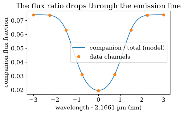
The primary is a point source with a unit continuum and a Brγ emission line three times as bright as the continuum at its peak. The companion has an OB star's continuum, a power law of index zero over this narrow band, wrapped in Scaled so that its one free parameter is comp.flux.ratio, the flux ratio at the reference wavelength. The data have four telescopes, two snapshots and nine channels across the line, with noise from a fixed seed. The printed numbers are the flux ratio in the continuum and at the line centre.
import warnings

warnings.filterwarnings("ignore")  # coarse demo grids trip the peak-resolution warnings

import jax
import numpy as onp
import matplotlib.pyplot as plt

from virgil import GaussianLine, OIData, PointSource, PowerLaw, Scaled, Sum, System
from virgil.coverage import vlti_oidata
from virgil.detection import detection_statistics
from virgil.grid_fit import linear_flux_grid
from virgil.limits import injection_limits
from virgil.plotting import plot_grid_map, set_style

set_style()
BRG, FWHM = 2.1661e-6, 1.5e-9
waves = onp.linspace(BRG - 3e-9, BRG + 3e-9, 9)
continuum = [(waves[0] - 1e-10, waves[1] + 1e-10), (waves[-2] - 1e-10, waves[-1] + 1e-10)]
line = [(waves[3] - 1e-10, waves[5] + 1e-10)]

def wr_system(ratio, dra=8.0, ddec=-5.0):
    star = PointSource(flux=Sum(continuum=PowerLaw(1.0, wavel0=BRG), brg=GaussianLine(3.0, BRG, FWHM)))
    comp = PointSource(dra=dra, ddec=ddec, flux=Scaled(PowerLaw(1.0, wavel0=BRG), ratio))
    return System(star=star, comp=comp)

def template(blocks=("v2", "t3", "visphi", "flux"), sigma_phi=0.01):
    """GRAVITY AT-like snapshots with zero data, as an OIData dictionary."""
    base = vlti_oidata(hour_angles_h=(-1.0, 1.0), wavelengths_m=waves, sigma_v2=0.01, sigma_cp_deg=0.5)
    n = base.u.size
    rec = dict(u=onp.asarray(base.u), v=onp.asarray(base.v), wavel=onp.asarray(base.wavel),
               frame=onp.asarray(base.frame), stations=onp.asarray(base.stations),
               vis=onp.ones(n), d_vis=onp.full(n, 0.01), phi=onp.zeros(base.phi.size),
               d_phi=onp.full(base.phi.size, onp.radians(0.5)), i_cps1=onp.asarray(base.i_cps1),
               i_cps2=onp.asarray(base.i_cps2), i_cps3=onp.asarray(base.i_cps3))
    if "v2" not in blocks:
        rec["vis"] = onp.full(n, onp.nan)
    if "t3" not in blocks:
        rec.update(i_cps1=None, i_cps2=None, i_cps3=None, phi=None, d_phi=None, cp_flag=False)
    if "visphi" in blocks:
        rec["visphi"] = dict(sample=onp.arange(n), value=onp.zeros(n), error=onp.full(n, sigma_phi))
    if "flux" in blocks:
        rows = onp.repeat(onp.arange(n // waves.size), waves.size)
        rec["flux"] = dict(wavel=onp.asarray(base.wavel), value=onp.ones(n), error=onp.full(n, 0.05), row=rows)
    return rec

def observe(truth, blocks=("v2", "t3", "visphi", "flux"), sigma_phi=0.01, seed=1):
    data = OIData(template(blocks, sigma_phi))
    if "flux" in blocks:
        data = data.with_flux_scale(scale=(1.0, 0.5))
    if "visphi" in blocks:
        data = data.with_continuum(continuum, lines=line)
    return data.with_model(truth, key=jax.random.PRNGKey(seed))

truth = wr_system(0.08)
data = observe(truth)
total = truth.total_spectrum(waves)
print(f"flux ratio in the continuum: {0.08:.3f}")
print(f"flux ratio at the line centre: {0.08 / float(total[4]):.3f}")
flux ratio in the continuum: 0.080
flux ratio at the line centre: 0.020
Per channel, the model predicts the system's total flux and the companion's fraction of it. The companion's flux is constant, but the line lifts the total, so the fraction falls from about 8 per cent in the continuum to about 2 per cent at the line centre. The differential phase measures that change, not the mean.
Plotting code
fig, ax = plt.subplots(figsize=(6, 3.5))
fine = onp.linspace(waves[0], waves[-1], 200)
fraction = 0.08 / truth.total_spectrum(fine)
ax.plot((fine - BRG) * 1e9, fraction, label="companion / total (model)")
ax.plot((waves - BRG) * 1e9, 0.08 / total, "o", label="data channels")
ax.set_xlabel("wavelength - 2.1661 µm (nm)")
ax.set_ylabel("companion flux fraction")
ax.set_title("The flux ratio drops through the emission line")
ax.legend()
plt.show()
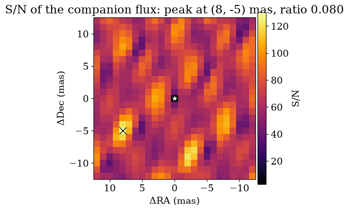
The quickest search is linear_flux_grid, which solves for the companion flux in closed form at every grid position. Give it a template whose companion has Scaled(...) with a starting ratio, and name the flux axis comp.flux.ratio: its values are ignored, but the key says which parameter is the flux. All four kinds of data enter the likelihood together. The map shows the signal-to-noise of the best flux at each position, the cross marks the injected position, and the printed numbers compare the recovered flux with the injected 0.08. This is a linearized search, not a fitted model, so there is no data-model correlation plot; the detection statistics below quantify the result.
axis = onp.arange(-12.0, 12.1, 1.0)
grid = {"comp.dra": axis, "comp.ddec": axis, "comp.flux.ratio": onp.array([0.0])}
search = linear_flux_grid(wr_system(0.05), data, grid, n_iter=3)
snr = onp.asarray(search.snr)
i, j = onp.unravel_index(onp.nanargmax(snr), snr.shape)
fig, ax = plt.subplots(figsize=(5, 4.5))
plot_grid_map(snr, grid={"dra": axis, "ddec": axis}, kind="snr", ax=ax)
ax.plot(8.0, -5.0, "kx", ms=10)
ax.set_title(f"S/N of the companion flux: peak at ({axis[i]:.0f}, {axis[j]:.0f}) mas, ratio {float(search.flux[i, j]):.3f}")
plt.show()
A search is only useful if you know what it could have seen. injection_limits adds a companion to the data at each position, with its chromatic signal in every observable, and reports the flux ratio at which the null model is rejected at 3σ. We evaluate it at a few separations along one direction, away from the companion already in the data at (8, −5) mas. The limits are on comp.flux.ratio, in the continuum; each position needs a bracketing search, hence the progress bar.
seps = onp.array([-10.0, -6.0, 0.0, 4.0])
limits = []
for dra in seps:
    point = {"comp.dra": onp.array([dra]), "comp.ddec": onp.array([-5.0]), "comp.flux.ratio": onp.array([0.01])}
    limits.append(float(injection_limits(wr_system(0.05), data, point, 3.0)[0, 0]))
for dra, limit in zip(seps, limits):
    print(f"dra = {dra:6.1f} mas: 3-sigma limit on the continuum flux ratio = {limit:.4f}")
dra =  -10.0 mas: 3-sigma limit on the continuum flux ratio = 0.0574
dra =   -6.0 mas: 3-sigma limit on the continuum flux ratio = 0.0118
dra =    0.0 mas: 3-sigma limit on the continuum flux ratio = 0.0115
dra =    4.0 mas: 3-sigma limit on the continuum flux ratio = 0.0154
Now the sub-resolution case, which is why the chromatic model matters. We move the companion to 0.1 mas, a fiftieth of the 4 mas resolution of a 130 m baseline, and search data simulated with the same seed in two ways. A chromatic search on the differential phases alone sees the shifting photocentre; a grey search on the V² and closure phases sees almost nothing, since those change only at second order or higher in the separation. Part of the gap is the setup rather than the line: the differential-phase errors (0.005 rad) are smaller than the closure-phase errors (0.0087 rad), and there are more phases per sample. The statistic is delta_chi2, the χ² improvement of the best companion on the grid, which for a null result is of order 1 to 10 because it is a maximum over positions and fluxes.
sep = 0.1
sub = wr_system(0.2, dra=sep, ddec=0.0)
differential = observe(sub, ("visphi",), sigma_phi=0.005, seed=2)
grey = observe(sub, ("v2", "t3"), seed=2)
axes = {"comp.dra": onp.array([-sep, 0.0, sep]), "comp.ddec": onp.zeros(1)}
ratios = onp.geomspace(0.05, 0.5, 8)
chromatic = detection_statistics(wr_system(0.1), differential, {**axes, "comp.flux.ratio": ratios})
constant = detection_statistics(System(star=PointSource(flux=Sum(continuum=PowerLaw(1.0, wavel0=BRG), brg=GaussianLine(3.0, BRG, FWHM))), comp=PointSource(flux=0.1)), grey, {**axes, "comp.flux": ratios})
print(f"differential phase, chromatic model: delta chi2 = {float(chromatic['delta_chi2']):.1f}")
print(f"V2 and closure phase, grey ratio:    delta chi2 = {float(constant['delta_chi2']):.1f}")
differential phase, chromatic model: delta chi2 = 65.7
V2 and closure phase, grey ratio:    delta chi2 = 1.3
The line turns a companion invisible to V² and closure phases into a clear detection in the differential phase, with the same channels and seed, helped by the smaller phase errors. On real data, run the full recipe on each star: a linear_flux_grid map to find candidates, injection_limits for what the data exclude, and detection_statistics with simulated null draws (see the detection-ROC tutorial) for a false-alarm probability. Throughout, comp.flux.ratio is the flux axis, and any fixed spectral shape, not only a power law, can serve as the companion's by wrapping it in Scaled.