Radio imaging from visibilities: a simulated tutorial

This tutorial takes a simulated ALMA-like observation from visibilities to an image: build a ComplexVisData, set up the calibration nuisances, start from CLEAN, then fit a pixel Image and compare it with the truth. Everything is synthetic and seeded, so it runs anywhere in about a minute on a laptop CPU. For real data, replace the simulation with ComplexVisData.read_ms; the radio interferometry guide and the CLEAN guide document each piece.

import warnings

warnings.filterwarnings("ignore", category=SyntaxWarning)  # a docstring in a dependency
warnings.filterwarnings("ignore", message="IProgress")

import jax
import matplotlib.pyplot as plt
import numpy as onp
import numpyro.distributions as dist
from matplotlib.colors import PowerNorm

from virgil import CalibrationNuisance, ComplexVisData, Image, fit, scenes
from virgil._geometry import image_visibilities
from virgil.imaging import MaxEntropy
from virgil.radio_clean import clean, restore

jax.config.update("jax_enable_x64", True)  # the Toeplitz χ² needs float64

Simulated data

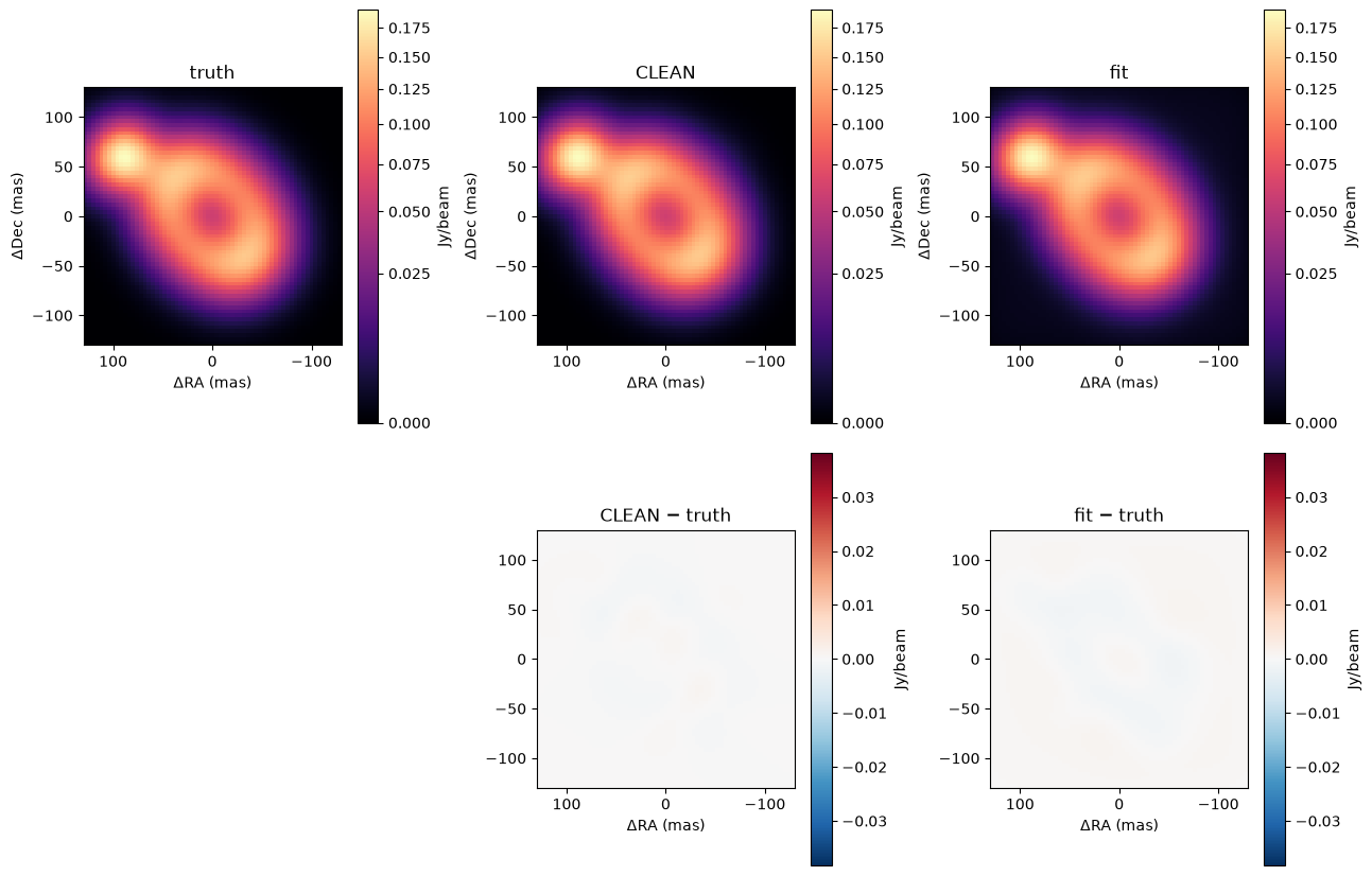
The truth is a 65 × 65 image of 4 mas pixels: an inclined ring of radius 60 mas holding 0.8 Jy, and a compact clump to its north-east holding 0.2 Jy. The observation tracks 300 random baselines for six hours (east and north components each log-uniform between 100 m and 10 km) at 1.3 mm from a southern site, giving 60,000 uv points. The visibilities are the exact transform of the truth plus Gaussian noise of 0.05 Jy per real and imaginary part.

N, S, SIG = 65, 4.0, 0.05  # pixels, mas per pixel, Jy per real/imaginary part
truth = onp.asarray(0.8 * scenes.ring(N, S, 60, 10, inc_deg=50, pa_deg=40) + 0.2 * scenes.gaussian_blob(N, S, 6, dra=90, ddec=60))
rng = onp.random.default_rng(1)
bl = onp.exp(rng.uniform(onp.log(100), onp.log(1e4), (300, 2))) * rng.choice([-1, 1], (300, 2))  # east, north (m)
H, dec, lat = onp.deg2rad(onp.linspace(-45, 45, 200)), onp.deg2rad(-37), onp.deg2rad(-23)
u = ((bl[:, :1] * onp.cos(H) - bl[:, 1:] * onp.sin(lat) * onp.sin(H)) / 1.3e-3).ravel()
v = ((bl[:, :1] * onp.sin(dec) * onp.sin(H) + bl[:, 1:] * (onp.sin(lat) * onp.sin(dec) * onp.cos(H) + onp.cos(lat) * onp.cos(dec))) / 1.3e-3).ravel()
vis = onp.asarray(image_visibilities(truth, u, v, S, ft="dft")) + SIG * (rng.normal(size=u.size) + 1j * rng.normal(size=u.size))

data = ComplexVisData.from_arrays(u, v, vis, 1 / SIG**2, 230e9)  # u, v in wavelengths; weight = 1/σ²
print(f"{len(data)} visibilities, longest baseline {onp.hypot(u, v).max() / 1e6:.1f} Mλ")

60000 visibilities, longest baseline 9.9 Mλ

Calibration nuisances

CalibrationNuisance configures what is fitted besides the sky. Here there is one observation with known errors, so only the total flux cal.flux is fitted: no gains, offsets, spectral index or error scales.

nuis = CalibrationNuisance(data, ref_obs=0, alpha=False, offsets=False, sigmas=False)
priors = nuis.priors()  # just cal.flux

A CLEAN start

radio_clean.clean gives a first image and its restoring beam (fit_beam fits the beam to the dirty beam's core). We compare reconstructions through that beam, which is what a perfect image would look like at this resolution.

sigma_img = 1 / onp.sqrt(onp.sum(onp.asarray(data.weight)))  # thermal noise of the natural-weighted image
res = clean(data, N, S, deconvolver="hogbom", threshold=3 * sigma_img, usemask="auto-multithresh")
print(f"CLEAN stopped on '{res.stop}' after {res.iterations} iterations; beam {res.beam[0]:.0f} x {res.beam[1]:.0f} mas")

CLEAN stopped on 'threshold' after 563 iterations; beam 49 x 46 mas

Fitting an Image

The scene is a pixel Image (the pixels are softmax(log_brightness), scaled by cal.flux), started from the CLEAN model. MaxEntropy regularizes it weakly. chi2="auto" is the default: because the scene is one fixed Image, with no antenna gains, offsets or fitted spectral index, in float64, with enough points per pixel, fit evaluates the exact Toeplitz form of χ² (a few FFTs of the image instead of a transform of 60,000 points), and info["likelihood_forms"] reports which form ran.

scene = lambda values: Image(values["log_brightness"], pixel_scale_mas=S)
start = onp.clip(res.model, 0, None) / onp.clip(res.model, 0, None).sum()
init = nuis.defaults()
init["log_brightness"] = onp.log(start + 1e-4 * start.max())
init["cal.flux"] = float(res.model.sum())
priors["log_brightness"] = dist.Normal(0.0, 3.0)

term = data.term(scene, nuis, chi2="auto")
result = fit(lambda **values: scene(values), priors, (), likelihoods=[term], regularizers=[MaxEntropy(1e3)],
             init=init, method="lbfgs", max_steps=5000)
print(result.info["likelihood_forms"], f"converged={result.info['converged']} in {result.info['steps']} steps")

['toeplitz'] converged=True in 2792 steps

The image against the truth

All panels are seen through the CLEAN beam, in Jy/beam. The last two are the CLEAN and fitted images minus the truth, on the same scale: signed residuals, with no uncertainties attached.

beam = res.beam
zeros = onp.zeros((N, N))
fit_image = onp.asarray(scene(result.values).brightness) * float(result.values["cal.flux"])
panels = {
    "truth": restore(truth, zeros, beam, S),
    "CLEAN": restore(res.model, zeros, beam, S),
    "fit": restore(fit_image, zeros, beam, S),
}
half = N * S / 2
fig, axes = plt.subplots(2, 3, figsize=(13, 8.5))
for ax, (name, im) in zip(axes[0], panels.items()):
    shown = ax.imshow(im, extent=[half, -half, -half, half], origin="upper", cmap="magma", norm=PowerNorm(0.5, vmin=0, vmax=panels["truth"].max()))
    ax.set(title=name, xlabel="ΔRA (mas)", ylabel="ΔDec (mas)")
    fig.colorbar(shown, ax=ax, label="Jy/beam")
lim = 0.2 * panels["truth"].max()
for ax, name in zip(axes[1, 1:], ("CLEAN", "fit")):
    shown = ax.imshow(panels[name] - panels["truth"], extent=[half, -half, -half, half], origin="upper", cmap="RdBu_r", vmin=-lim, vmax=lim)
    ax.set(title=f"{name} − truth", xlabel="ΔRA (mas)")
    fig.colorbar(shown, ax=ax, label="Jy/beam")
axes[1, 0].axis("off")
fig.tight_layout()

Diagnostics

The fit statistic is the raw χ² per datum on the quoted errors, Σ w |V − M|² / (2N) (two real numbers per visibility), which should be near 1 for a model that fits noise-limited data; it is not rescaled. We also report the flux and the rms difference from the truth through the beam, relative to the truth's peak.

w = onp.asarray(data.weight)
def chi2_per_datum(model_vis):
    return float(onp.sum(w * onp.abs(onp.asarray(data.vis) - model_vis) ** 2) / (2 * len(data)))

fit_vis = onp.asarray(data.model(scene(result.values), result.values, nuis))
peak = panels["truth"].max()
for name, model_vis, im, flux in (("CLEAN", res.model_visibilities(data), panels["CLEAN"], res.model.sum()),
                                  ("fit", fit_vis, panels["fit"], fit_image.sum())):
    print(f"{name:5s} χ²/N = {chi2_per_datum(onp.asarray(model_vis)):.3f}, flux {flux:.3f} Jy (true {truth.sum():.3f}), "
          f"rms − truth {onp.sqrt(onp.mean((im - panels['truth']) ** 2)) / peak:.3f} of peak")
print(f"fit reports χ² = {result.info['chi2'][0]:.0f} for {int(result.info['ndata'][0])} data")

CLEAN χ²/N = 1.005, flux 0.999 Jy (true 1.000), rms − truth 0.002 of peak
fit   χ²/N = 1.003, flux 1.008 Jy (true 1.000), rms − truth 0.003 of peak
fit reports χ² = 120350 for 120000 data

Notes

The fit used the default exact path. Fitted phase-centre offsets would need offsets="spread" in ComplexVisData.toeplitz, an opt-in extension that is derived here, not published; antenna gains and a fitted spectral index fall back to the direct transform. The package is provisional, so details may change before it settles. See the radio interferometry guide for the model, the nuisances and the Toeplitz χ², and the CLEAN guide for clean.